一、準備工作

電腦發出數據的波形圖繪制在我的另一篇博客有詳細介紹：

根據Wireshark捕獲數據包時間和長度繪制電腦發射信號波形-CSDN博客

路由器發送給電腦數據的波形圖繪制也在我的另一篇博客有詳細介紹：

根據Wireshark捕獲數據包時間和長度繪制路由器發送給電腦數據的信號波形-CSDN博客

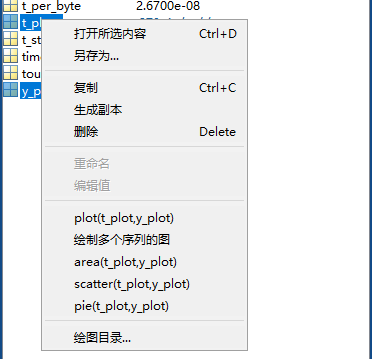
這里額外介紹了下怎么便捷保存MATLAB變量，可以用來保存繪制的電腦發射信號波形數據和路由器發射信號波形數據：
MATLAB變量便捷存儲方法-CSDN博客

二、比較波形繪制

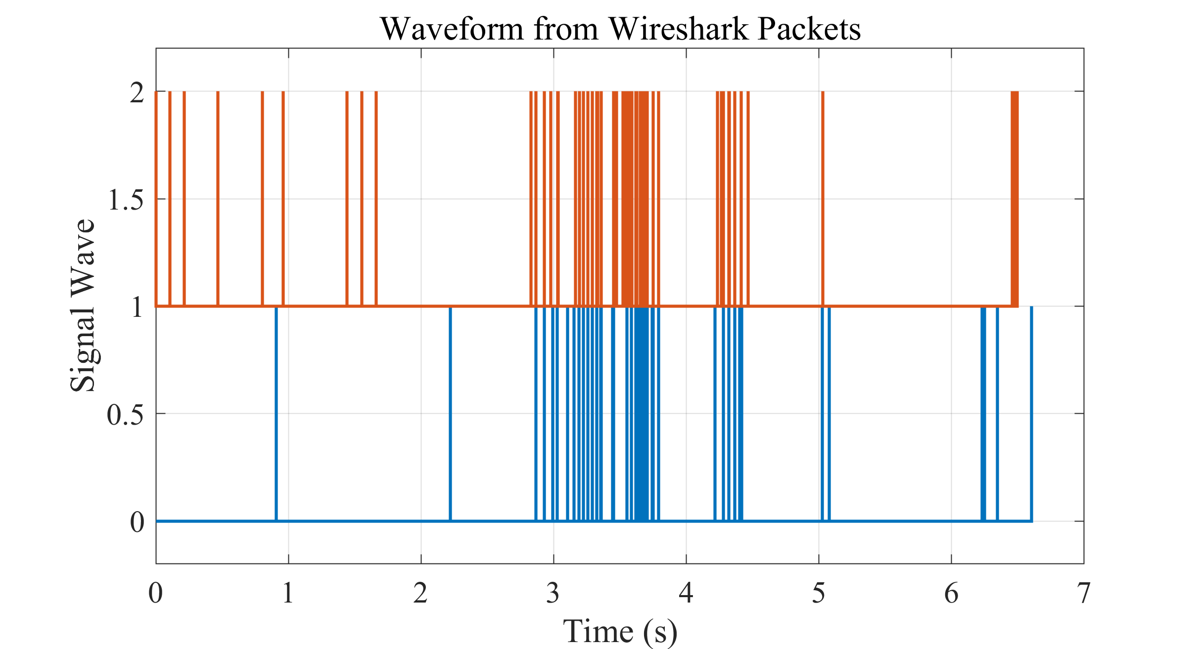
本篇文章把兩個波形圖繪制在一起，進行比較。程序：

%zhouzhichao
%2025年8月20日
%觀察路由器、電腦互相發送的信號
clc
close all
clear
load("D:\無線通信網絡認知\通信學報\5G信號\Wireshark波形繪制\direction_192_168_1_103.mat")
y_plot_1 = y_plot;
t_plot_1 = t_plot;
load("D:\無線通信網絡認知\通信學報\5G信號\Wireshark波形繪制\source_192_168_1_103.mat")
y_plot_2 = y_plot;
t_plot_2 = t_plot;%% 繪圖
figure; 
stairs(t_plot_1, y_plot_1, 'LineWidth', 1.5);
hold on
y_plot_2=y_plot_2+1;
stairs(t_plot_2, y_plot_2, 'LineWidth', 1.5);ylim([-0.2 2.2]);
xlabel('Time (s)');
ylabel('Signal Wave');
title('Waveform from Wireshark Packets');
grid on;set(gca, 'FontName', 'Times New Roman')
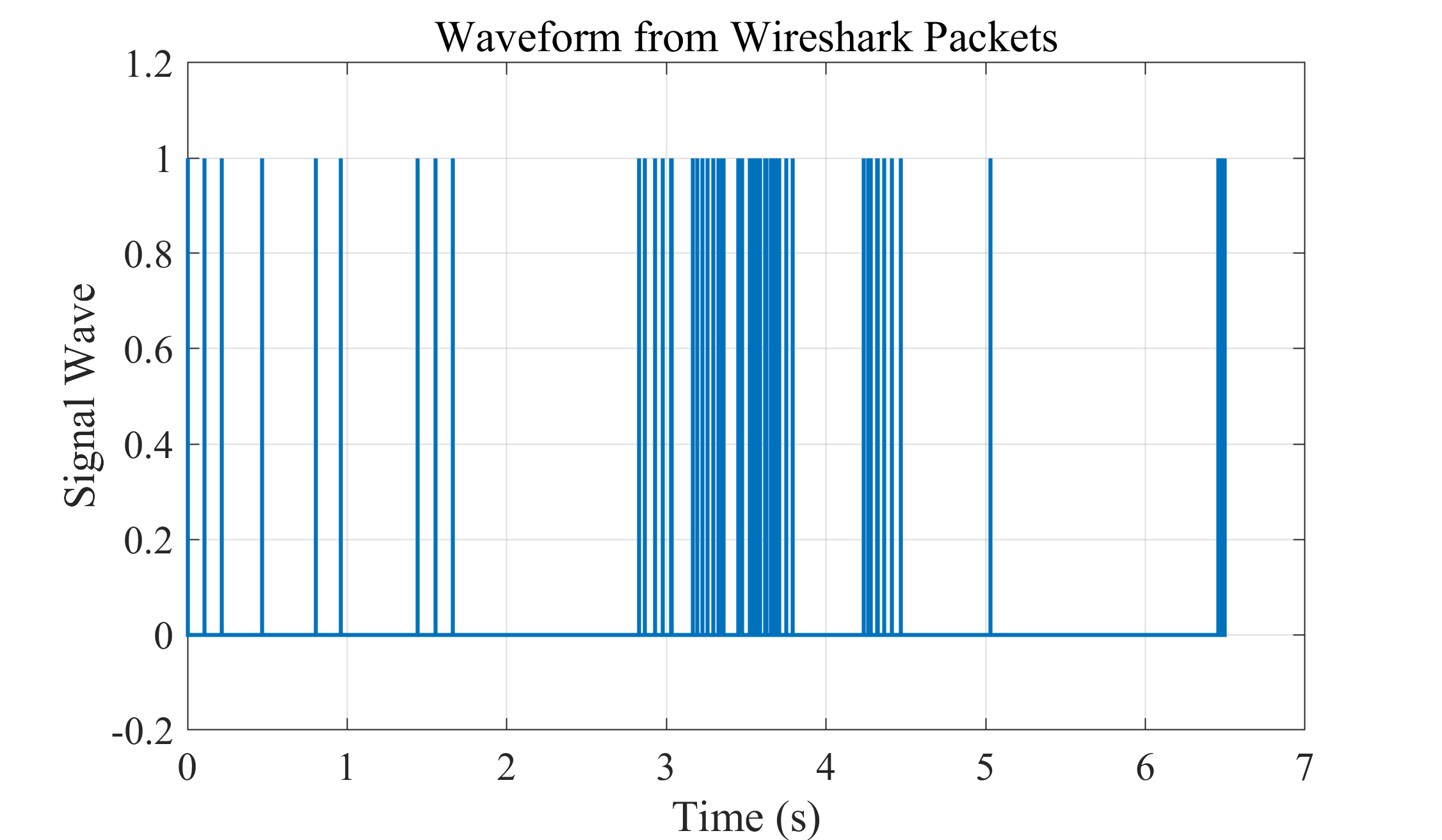
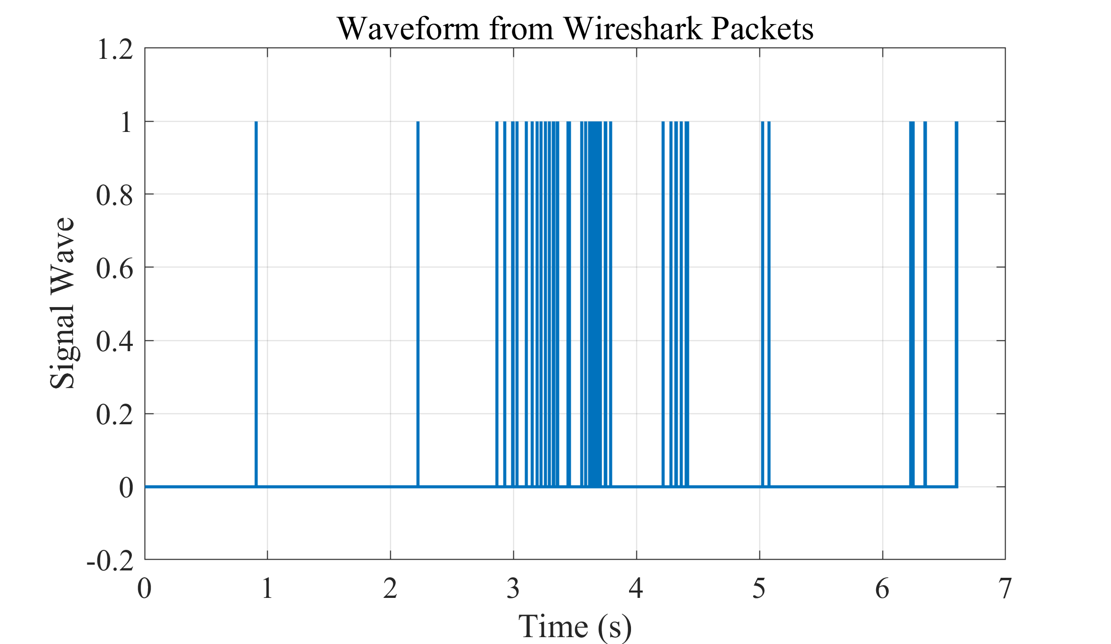
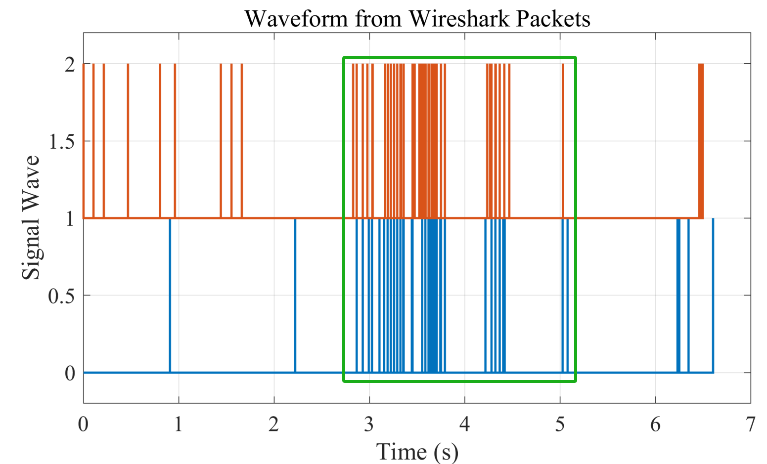
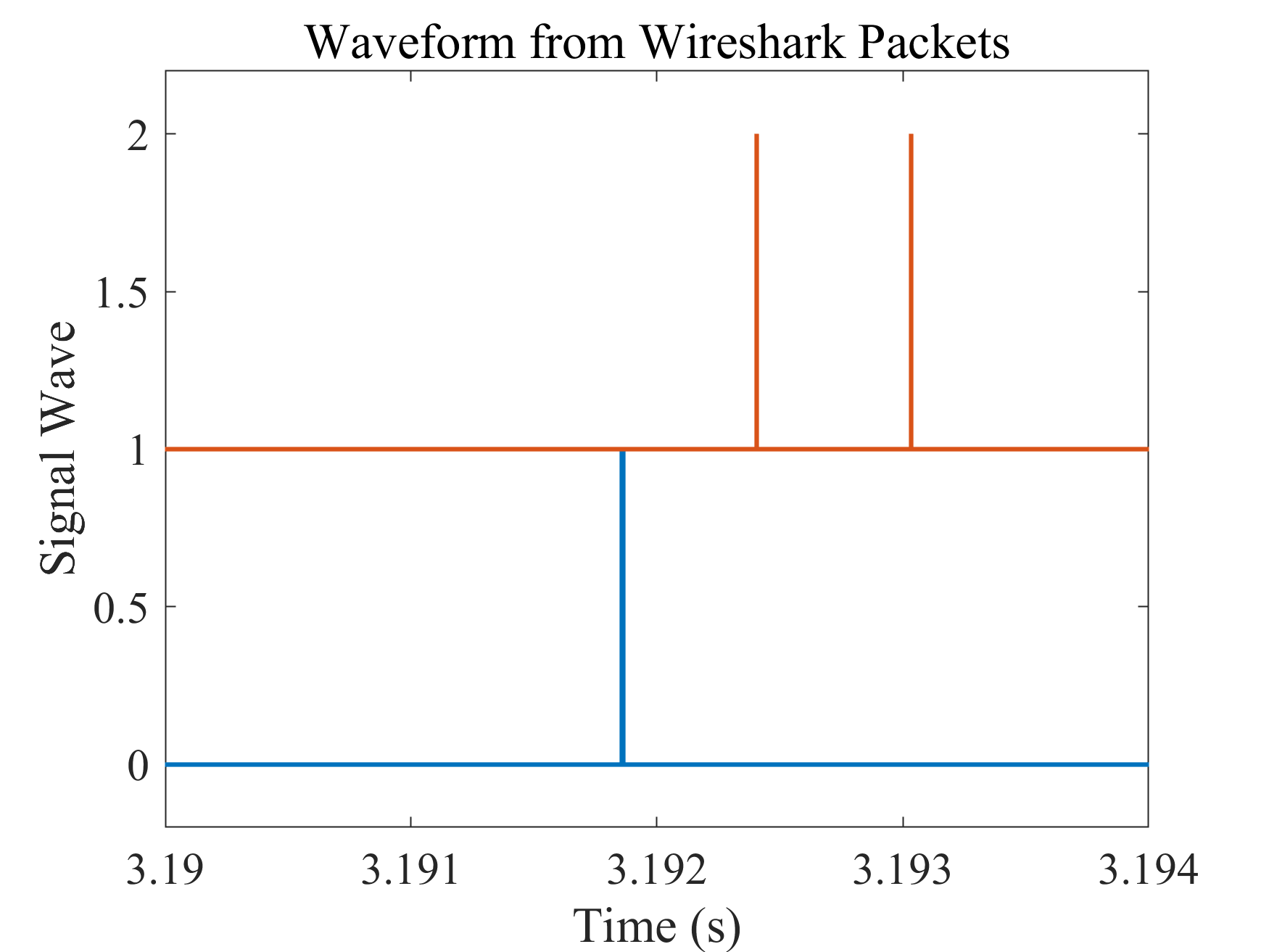
set(gca, 'FontSize', 15)save("D:\無線通信網絡認知\通信學報\5G信號\Wireshark波形繪制\save_test.mat","t_plot","y_plot")

source=192.168.1.103的波形和direction=192.168.1.103的波形，其中上面是我的電腦發出的信號波形，下面是我的電腦收到的信號波形（路由器發送）：

三、波形多尺度觀察

綠色框里電腦和路由器的波形表現出明顯的相互性：

但是黃色框里電腦和路由器的波形顯現得比較獨立：

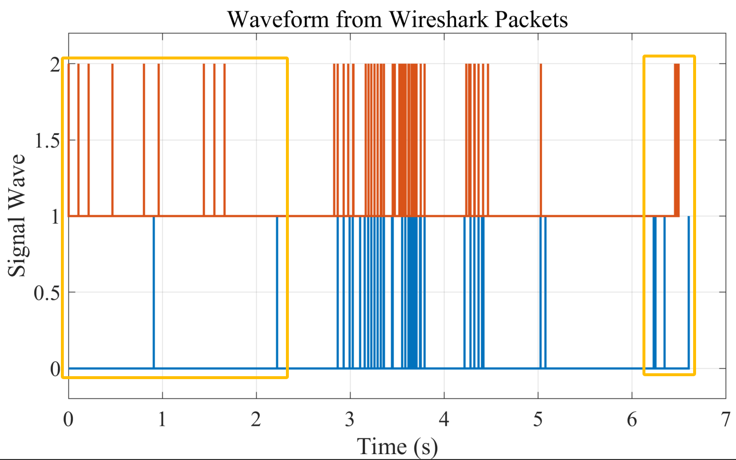
最前面我的電腦（紅色）發了好多波形，路由器沒響應；最后這個其實響應還比較明顯，路由器（藍色）發了很多數據，電腦收到后逐個響應。

放大波形看看：

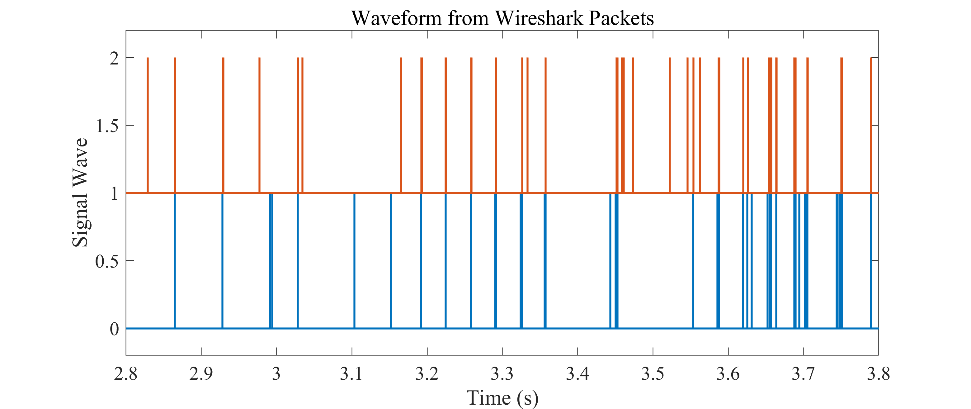
[3.1, 3.3]

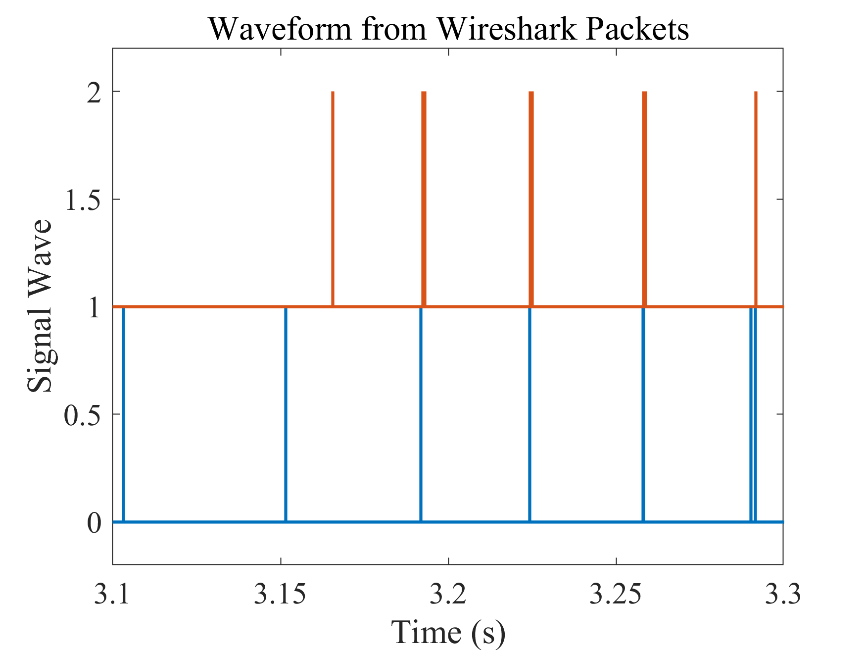
[3.19, 3.194]

xlim([3.19184,3.19187])

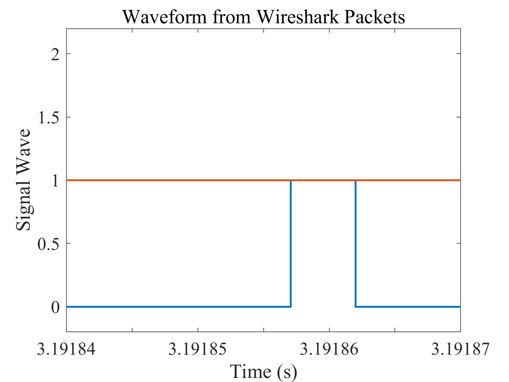
四、搭上載波

[3.19184,3.19187]這段信號時長3.19187-3.19184=0.00003s=0.03ms=30ns

2.4GHz下設置24GHz的采樣率的話

0.00003s*24GHz=0.00003*24*10^9=720000采樣點=72萬個采樣點

試試能不能仿真出來：

4.1 截取信號

首先把y_plot_1，t_plot_1在[3.19184,3.19187]進行截取：

%% 截取信號
% 定義時間區間
t_start = 3.19184;
t_end = 3.19187;% 找到在這個時間區間內的索引
indices = t_plot_1 >= (t_start-0.1) & t_plot_1 <= (t_end+0.1);% 截取數據
t_plot_1_segment = t_plot_1(indices);
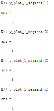
y_plot_1_segment = y_plot_1(indices);% 繪制截取后的波形
figure;
stairs(t_plot_1_segment, y_plot_1_segment, 'LineWidth', 1.5);
xlim([t_start, t_end]);
ylim([-0.2, 2.2]);
xlabel('Time (s)');
ylabel('Signal Wave');
title('Segmented Waveform from Wireshark Packets');
set(gca, 'FontName', 'Times New Roman');
set(gca, 'FontSize', 15);

再繪制波形：

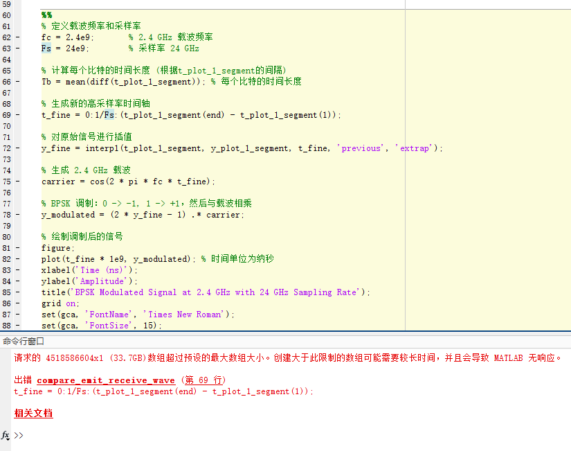
MATLAB直接仿真2.4GHz的載波有些太困難了。

降低采樣率：

% 定義載波頻率和采樣率
fc = 2.4e9;       % 2.4 GHz 載波頻率
Fs = 5e9;        % 采樣率 24 GHz

4.2 時間軸遞增

K>> fprintf('%.8f\n', t_plot_1_segment(1));
3.10319956
K>> fprintf('%.8f\n', t_plot_1_segment(2));
3.10319956
K>> fprintf('%.8f\n', t_plot_1_segment(3));
3.10320100
K>> fprintf('%.8f\n', t_plot_1_segment(4));
3.10320100

把t軸上一樣的數值第一次出現時-0.00001：

% 初始偏移量
offset = 0.00001;% 初始化一個新數組，用于存儲調整后的值
t_plot_1_segment_adjusted = t_plot_1_segment;% 遍歷 `t_plot_1_segment` 數組
for i = 2:length(t_plot_1_segment)% 如果當前值與前一個值相同，調整當前值if t_plot_1_segment_adjusted(i) == t_plot_1_segment_adjusted(i-1)t_plot_1_segment_adjusted(i-1) = t_plot_1_segment_adjusted(i-1) - offset;end
end

4.3 插值

插值思路：

對y_plot_1_segment和t_plot_1_segment_adjusted進行插值。

首先檢查y_plot_1_segment中的兩個挨在一起的1，中間補充1，補充1的數量根據兩個挨在一起的1對應的t_plot_1_segment_adjusted中的數值差，和采樣率Fs計算；

然后，檢查y_plot_1_segment中的兩個挨在一起的0，中間補充0，補充0的數量根據兩個挨在一起的0對應的t_plot_1_segment_adjusted中的數值差，和采樣率Fs計算；

最后，檢查y_plot_1_segment中的兩個挨在一起的0和1，0和1之間補充0，補充0的數量根據兩個挨在一起的0對應的t_plot_1_segment_adjusted中的數值差，和采樣率Fs計算。

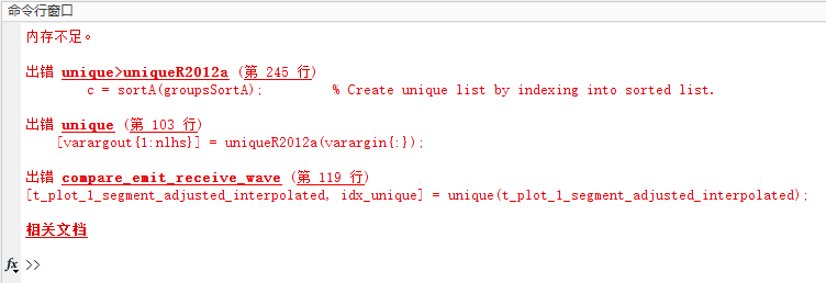
內存還是不夠，降低中心頻率和采樣率：

% 定義載波頻率和采樣率
fc = 1.2e9;       % 2.4 GHz 載波頻率
Fs = 39;        % 采樣率 24 GHz

4.4 電磁波

本來還想在調制載波之后優化為電磁波圖：

(27 封私信) 用什么軟件能畫出這樣的圖？ - 知乎

x = (0:2:300)/50;
y = -sin(x*pi); z = cos(x*pi);
[m,M] = cellfun(@(t)deal(min(t),max(t)),{x,y,z});
[yc,zc,xc] = cylinder(1,500); xc = xc*M(1);
figure('render','painter','color','w'), view(44,14), axis image ij off, hold on
line(x,y,z,'linewidth',2,'color','r')
line(xc',yc',zc','color',[1 0.7 0.7])
h = surface(xc,yc,zc,'facecolor','none','edgecolor','r','edgealpha',0.02);
quiver3(x,0*x,0*z,0*x,y,z,0,'k','linewidth',1,'maxhead',0.06);
quiver3([m(1) 0 0],[0 m(2) 0],[0 0 m(3)],...[1.2*(M(1)-m(1)) 0 0],[0 1.3*(M(2)-m(2)) 0],[0 0 1.3*(M(3)-m(3))],0,...'linewidth',2,'color','k','maxhead',0.08)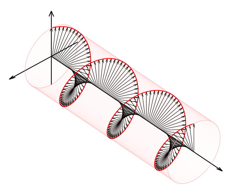

現在連載波也仿真不出。