目錄
- 1 時空解耦運動規劃
- 2 PJSO速度規劃原理
- 2.1 優化變量
- 2.2 代價函數
- 2.3 約束條件
- 2.4 二次規劃形式
- 3 算法仿真
- 3.1 ROS C++仿真
- 3.2 Python仿真
1 時空解耦運動規劃
在自主移動系統的運動規劃體系中,時空解耦的遞進式架構因其高效性與工程可實現性被廣泛采用。這一架構將復雜的高維運動規劃問題分解為路徑規劃與速度規劃兩個層次化階段:路徑規劃階段基于靜態環境約束生成無碰撞的幾何軌跡;速度規劃階段則在此基礎上引入時間維度,通過動態障礙物預測、運動學約束建模等為機器人或車輛賦予時間軸上的運動規律。這種解耦策略雖在理論上犧牲了時空聯合優化的最優性,卻通過分層降維大幅提升了復雜場景下的計算效率,使其成為自動駕駛、服務機器人等實時系統的經典方案。

2 PJSO速度規劃原理
2.1 優化變量
分段加加速度優化(Piecewise Jerk Speed Optimizer, PJSO)算法是常用的縱向速度優化方式,核心原理是用三次多項式表示s-t圖中每個時間區間 [ t k , t k + 1 ) \left[ t_k,t_{k+1} \right) [tk?,tk+1?)的速度曲線,并約束每個區間加加速度相等,其中 k = 0 , 1 , ? , n ? 2 k=0,1,\cdots ,n-2 k=0,1,?,n?2, 可取為路徑規劃的路點數量。PJSO算法的優化變量為
x = [ l s 0 s ˙ 0 s ¨ 0 ? s k s ˙ k s ¨ k ? s n ? 1 s ˙ n ? 1 s ¨ n ? 1 ] 3 n × 1 T \boldsymbol{x}=\left[ \begin{matrix}{l} s_0& \dot{s}_0& \ddot{s}_0& \cdots& s_k& \dot{s}_k& \ddot{s}_k& \cdots& s_{n-1}& \dot{s}_{n-1}& \ddot{s}_{n-1}\\\end{matrix} \right] _{3n\times 1}^{T} x=[ls0??s˙0??s¨0????sk??s˙k??s¨k????sn?1??s˙n?1??s¨n?1??]3n×1T?
2.2 代價函數
代價函數可設計為
J = ∑ i = 0 n ? 2 ( w s ( s i ? s i , r e f ) 2 + w v ( s ˙ i ? s ˙ i , r e f ) 2 + w a s ¨ i 2 + w j s i ( 3 ) 2 ) + w s , e n d ( s n ? 1 ? s e n d ) 2 + w v , e n d ( s ˙ n ? 1 ? s ˙ e n d ) 2 + w a , e n d ( s ¨ n ? s ¨ e n d ) 2 J=\sum_{i=0}^{n-2}{\left( w_s\left( s_i-s_{i,\mathrm{ref}} \right) ^2+w_v\left( \dot{s}_i-\dot{s}_{i,\mathrm{ref}} \right) ^2+w_a\ddot{s}_{i}^{2}+w_j{s}_{i}^{(3)2} \right)}\\+w_{s,\mathrm{end}}\left( s_{n-1}-s_{\mathrm{end}} \right) ^2+w_{v,\mathrm{end}}\left( \dot{s}_{n-1}-\dot{s}_{\mathrm{end}} \right) ^2+w_{a,\mathrm{end}}\left( \ddot{s}_n-\ddot{s}_{\mathrm{end}} \right) ^2 J=i=0∑n?2?(ws?(si??si,ref?)2+wv?(s˙i??s˙i,ref?)2+wa?s¨i2?+wj?si(3)2?)+ws,end?(sn?1??send?)2+wv,end?(s˙n?1??s˙end?)2+wa,end?(s¨n??s¨end?)2
通過
s i ( 3 ) = s ¨ i + 1 ? s ¨ i Δ t {s}_i^{(3)}=\frac{\ddot{s}_{i+1}-\ddot{s}_i}{\Delta t} si(3)?=Δts¨i+1??s¨i??
隱式地消除加加速度變量,代入代價函數并消除常數項可化簡為
J = w s ∑ i = 0 n ? 2 s i 2 + w s , e n d s n ? 1 2 ? 2 w s ∑ i = 0 n ? 2 s i , r e f s i ? 2 w s , e n d s e n d s n ? 1 + w v ∑ i = 0 n ? 2 s ˙ i 2 + w v , e n d s ˙ n ? 1 2 ? 2 w v ∑ i = 0 n ? 2 s ˙ i , r e f s ˙ i ? 2 w v , e n d s ˙ e n d s ˙ n ? 1 + ( w a + w j Δ t 2 ) s ¨ 0 2 + ( w a + w a , e n d + w j Δ t 2 ) s ¨ n ? 1 2 ? 2 w a , e n d s ¨ e n d s ¨ n ? 1 + ( w a + 2 w j Δ t 2 ) ∑ i = 1 n ? 2 s ¨ i 2 ? 2 w j Δ t 2 ∑ i = 0 n ? 2 s ¨ i s ¨ i + 1 \begin{aligned}J=&w_s\sum_{i=0}^{n-2}{s_{i}^{2}}+w_{s,\mathrm{end}}s_{n-1}^{2}-2w_s\sum_{i=0}^{n-2}{s_{i,\mathrm{ref}}s_i}-2w_{s,\mathrm{end}}s_{\mathrm{end}}s_{n-1}\\&+w_v\sum_{i=0}^{n-2}{\dot{s}_{i}^{2}}+w_{v,\mathrm{end}}\dot{s}_{n-1}^{2}-2w_v\sum_{i=0}^{n-2}{\dot{s}_{i,\mathrm{ref}}\dot{s}_i}-2w_{v,\mathrm{end}}\dot{s}_{\mathrm{end}}\dot{s}_{n-1}\\&+\left( w_a+\frac{w_j}{\Delta t^2} \right) \ddot{s}_{0}^{2}+\left( w_a+w_{a,\mathrm{end}}+\frac{w_j}{\Delta t^2} \right) \ddot{s}_{n-1}^{2}-2w_{a,\mathrm{end}}\ddot{s}_{\mathrm{end}}\ddot{s}_{n-1}\\&+\left( w_a+\frac{2w_j}{\Delta t^2} \right) \sum_{i=1}^{n-2}{\ddot{s}_{i}^{2}}-\frac{2w_j}{\Delta t^2}\sum_{i=0}^{n-2}{\ddot{s}_i\ddot{s}_{i+1}}\end{aligned} J=?ws?i=0∑n?2?si2?+ws,end?sn?12??2ws?i=0∑n?2?si,ref?si??2ws,end?send?sn?1?+wv?i=0∑n?2?s˙i2?+wv,end?s˙n?12??2wv?i=0∑n?2?s˙i,ref?s˙i??2wv,end?s˙end?s˙n?1?+(wa?+Δt2wj??)s¨02?+(wa?+wa,end?+Δt2wj??)s¨n?12??2wa,end?s¨end?s¨n?1?+(wa?+Δt22wj??)i=1∑n?2?s¨i2??Δt22wj??i=0∑n?2?s¨i?s¨i+1??
從而得到核矩陣
P = [ P s P s ˙ P s ¨ ] 3 n × 3 n \boldsymbol{P}=\left[ \begin{matrix} \boldsymbol{P}_s& & \\ & \boldsymbol{P}_{\dot{s}}& \\ & & \boldsymbol{P}_{\ddot{s}}\\\end{matrix} \right] _{3n\times 3n} P=???Ps??Ps˙??Ps¨?????3n×3n?
和偏置向量
q = [ ? 2 w s s 0 , r e f ? ? 2 w s s n ? 2 , r e f ? 2 w s , e n d s e n d ? 2 w v s ˙ 0 , r e f ? ? 2 w v s ˙ n ? 2 , r e f ? 2 w v , e n d s ˙ e n d 0 ? 0 ? 2 w a , e n d s ¨ e n d ] 3 n × 1 \boldsymbol{q}=\left[ \begin{array}{c} -2w_ss_{0,\mathrm{ref}}\\ \vdots\\ -2w_ss_{n-2,\mathrm{ref}}\\ -2w_{s,\mathrm{end}}s_{\mathrm{end}}\\ \hline -2w_v\dot{s}_{0,\mathrm{ref}}\\ \vdots\\ -2w_v\dot{s}_{n-2,\mathrm{ref}}\\ -2w_{v,\mathrm{end}}\dot{s}_{\mathrm{end}}\\ \hline 0\\ \vdots\\ 0\\ -2w_{a,\mathrm{end}}\ddot{s}_{\mathrm{end}}\\\end{array} \right] _{3n\times 1} q=?????????????????????????2ws?s0,ref???2ws?sn?2,ref??2ws,end?send??2wv?s˙0,ref???2wv?s˙n?2,ref??2wv,end?s˙end?0?0?2wa,end?s¨end???????????????????????????3n×1?
2.3 約束條件
根據運動學公式可得運動學等式約束
{ s ˙ i + 1 = s ˙ i + s ¨ i Δ t + 1 2 j i Δ t 2 = s ˙ i + 1 2 s ¨ i Δ t + 1 2 s ¨ i + 1 Δ t s i + 1 = s i + s ˙ i Δ t + 1 2 s ¨ i Δ t 2 + 1 6 j i Δ t 3 = s i + s ˙ i Δ t + 1 3 s ¨ i Δ t 2 + 1 6 s ¨ i + 1 Δ t 3 \begin{cases} \dot{s}_{i+1}=\dot{s}_i+\ddot{s}_i\Delta t+\frac{1}{2}j_i\Delta t^2=\dot{s}_i+\frac{1}{2}\ddot{s}_i\Delta t+\frac{1}{2}\ddot{s}_{i+1}\Delta t\\ s_{i+1}=s_i+\dot{s}_i\Delta t+\frac{1}{2}\ddot{s}_i\Delta t^2+\frac{1}{6}j_i\Delta t^3=s_i+\dot{s}_i\Delta t+\frac{1}{3}\ddot{s}_i\Delta t^2+\frac{1}{6}\ddot{s}_{i+1}\Delta t^3\\\end{cases} {s˙i+1?=s˙i?+s¨i?Δt+21?ji?Δt2=s˙i?+21?s¨i?Δt+21?s¨i+1?Δtsi+1?=si?+s˙i?Δt+21?s¨i?Δt2+61?ji?Δt3=si?+s˙i?Δt+31?s¨i?Δt2+61?s¨i+1?Δt3?
約束初始狀態
s ˙ 0 = s ˙ i n i t , s ˙ 0 = s ˙ i n i t , s ¨ 0 = s ¨ i n i t \dot{s}_0=\dot{s}_{\mathrm{init}}, \dot{s}_0=\dot{s}_{\mathrm{init}}, \ddot{s}_0=\ddot{s}_{\mathrm{init}} s˙0?=s˙init?,s˙0?=s˙init?,s¨0?=s¨init?
此外還需保證各階狀態量滿足不等式約束
s min ? ? s i ? s max ? , s ˙ min ? ? s ˙ i ? s ˙ max ? , s ¨ min ? ? s ¨ i ? s ¨ max ? , s ¨ min ? ( 3 ) Δ t ? s ¨ i + 1 ? s ¨ i ? s ¨ max ? ( 3 ) Δ t s_{\min}\leqslant s_i\leqslant s_{\max}, \dot{s}_{\min}\leqslant \dot{s}_i\leqslant \dot{s}_{\max}, \ddot{s}_{\min}\leqslant \ddot{s}_i\leqslant \ddot{s}_{\max}, \ddot{s}_{\min}^{(3)}\Delta t\leqslant \ddot{s}_{i+1}-\ddot{s}_i\leqslant \ddot{s}_{\max}^{(3)}\Delta t smin??si??smax?,s˙min??s˙i??s˙max?,s¨min??s¨i??s¨max?,s¨min(3)?Δt?s¨i+1??s¨i??s¨max(3)?Δt
從而得到約束矩陣
A = [ A i n i t , 3 × 3 n A b o u n d , 3 n + ( n ? 1 ) × 3 n A s y s , 2 ( n ? 1 ) × 3 n ] 6 n × 3 n , l = [ l i n i t l b o u n d l s y s ] 6 n × 1 , u = [ u i n i t u b o u n d u s y s ] 6 n × 1 \boldsymbol{A}=\left[ \begin{array}{c} \boldsymbol{A}_{\mathrm{init}, 3\times 3n}\\ \boldsymbol{A}_{\mathrm{bound}, 3n+\left( n-1 \right) \times 3n}\\ \boldsymbol{A}_{\mathrm{sys}, 2\left( n-1 \right) \times 3n}\\\end{array} \right] _{6n\times 3n}, \boldsymbol{l}=\left[ \begin{array}{c} \boldsymbol{l}_{\mathrm{init}}\\ \boldsymbol{l}_{\mathrm{bound}}\\ \boldsymbol{l}_{\mathrm{sys}}\\\end{array} \right] _{6n\times 1}, \boldsymbol{u}=\left[ \begin{array}{c} \boldsymbol{u}_{\mathrm{init}}\\ \boldsymbol{u}_{\mathrm{bound}}\\ \boldsymbol{u}_{\mathrm{sys}}\\\end{array} \right] _{6n\times 1} A=???Ainit,3×3n?Abound,3n+(n?1)×3n?Asys,2(n?1)×3n?????6n×3n?,l=???linit?lbound?lsys?????6n×1?,u=???uinit?ubound?usys?????6n×1?
2.4 二次規劃形式
綜上所述,可得到PJSO算法的二次規劃形式
min ? x J = x T P x + q T x s . t . l ? A x ? u \min _{\boldsymbol{x}}J=\boldsymbol{x}^T\boldsymbol{Px}+\boldsymbol{q}^T\boldsymbol{x}\\\mathrm{s}.\mathrm{t}. \boldsymbol{l}\leqslant \boldsymbol{Ax}\leqslant \boldsymbol{u} xmin?J=xTPx+qTxs.t.l?Ax?u
3 算法仿真
3.1 ROS C++仿真
核心代碼如下所示:
bool PiecewiseJerkVelocityPlanner::plan(const Points3d& waypoints, VelocityProfile& velocity_profile)
{int dim = static_cast<int>(waypoints.size());std::vector<double> s_ref(dim, 0.0);for (int i = 1; i < dim; ++i){s_ref[i] =s_ref[i - 1] + std::hypot(waypoints[i].x() - waypoints[i - 1].x(), waypoints[i].y() - waypoints[i - 1].y());}x_max_ = s_ref.back();// construct QP ProblemEigen::MatrixXd P, A;std::vector<c_float> l, u, q;_calKernel(dim, P);_calOffset(dim, s_ref, q);_calAffineConstraint(dim, A);_calBoundary(dim, s_ref, l, u);std::vector<c_float> P_data;std::vector<c_int> P_indices;std::vector<c_int> P_indptr;int ind_P = 0;for (int col = 0; col < P.cols(); ++col){P_indptr.push_back(ind_P);for (int row = 0; row <= col; ++row){P_data.push_back(P(row, col));P_indices.push_back(row);ind_P++;}}P_indptr.push_back(ind_P);std::vector<c_float> A_data;std::vector<c_int> A_indices;std::vector<c_int> A_indptr;int ind_A = 0;for (int col = 0; col < A.cols(); ++col){A_indptr.push_back(ind_A);for (int row = 0; row < A.rows(); ++row){double data = A(row, col);if (std::fabs(data) > kMathEpsilon){A_data.push_back(data);A_indices.push_back(row);++ind_A;}}}A_indptr.push_back(ind_A);// solveOSQPWorkspace* work = nullptr;OSQPData* data = reinterpret_cast<OSQPData*>(c_malloc(sizeof(OSQPData)));OSQPSettings* settings = reinterpret_cast<OSQPSettings*>(c_malloc(sizeof(OSQPSettings)));osqp_set_default_settings(settings);settings->verbose = false;settings->warm_start = true;data->n = 3 * dim;data->m = 6 * dim;data->P = csc_matrix(data->n, data->n, P_data.size(), P_data.data(), P_indices.data(), P_indptr.data());data->A = csc_matrix(data->m, data->n, A_data.size(), A_data.data(), A_indices.data(), A_indptr.data());data->q = q.data();data->l = l.data();data->u = u.data();osqp_setup(&work, data, settings);osqp_solve(work);auto status = work->info->status_val;if ((status < 0) || (status != 1 && status != 2)){R_DEBUG << "failed optimization status: " << work->info->status;return false;}// parsefor (int i = 0; i < dim; ++i){velocity_profile.push(dt_ * i, work->solution->x[i], work->solution->x[dim + i], work->solution->x[2 * dim + i]);}// Cleanuposqp_cleanup(work);c_free(data->A);c_free(data->P);c_free(data);c_free(settings);return true;
}
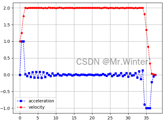
這里設置初始速度 v 0 = 1.0 m / s v_0=1.0\ m/s v0?=1.0?m/s,初始加速度 a 0 = 0 m / s 2 a_0=0\ m/s^2 a0?=0?m/s2;終點速度 v 0 = 0.0 m / s v_0=0.0\ m/s v0?=0.0?m/s,終點加速度 a 0 = 0 m / s 2 a_0=0\ m/s^2 a0?=0?m/s2
3.2 Python仿真
核心代碼如下所示:
def process(self, path: List[Point3d]) -> List[Dict]:velocity_profiles = []path_segs, path_refs = PathPlanner.getPathSegments(path)for i, path_seg in enumerate(path_segs):s_ref = path_refs[i]n = max(len(path_refs[i]),round(self.r * (self.dx_max ** 2 + s_ref[-1] * self.ddx_max) \/ (self.dx_max * self.ddx_max * self.dt)))s_ref = np.linspace(0, s_ref[-1], n)'''min x^T P x + q^T xs.t. l <= Ax <= u'''P = sparse.csc_matrix(self.calKernel(n))q = self.calOffset(n, s_ref)A = sparse.csc_matrix(self.calAffineConstraint(n))l, u = self.calBoundary(n, s_ref)solver = osqp.OSQP()solver.setup(P, q, A, l, u, verbose=False)res = solver.solve()sol = res.xvelocity_profiles.append({"time": [self.dt * i for i in range(n)],"path": PathPlanner.pathInterpolation(path_seg, n),"distance": sol[:n].tolist(),"velocity": sol[n:2 * n].tolist(),"acceleration": sol[2 * n:3 * n].tolist(),})return velocity_profiles
對于如下圖所示的倒車路徑
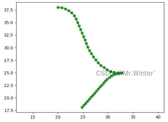
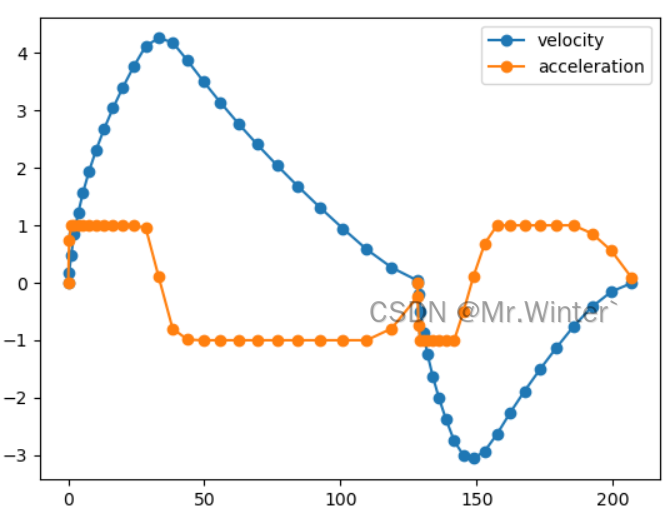
規劃的速度和加速度曲線如下所示,中間速度為0處為換擋點
🔥 更多精彩專欄:
- 《ROS從入門到精通》
- 《Pytorch深度學習實戰》
- 《機器學習強基計劃》
- 《運動規劃實戰精講》
- …


)


)


—— 內存優化)


