基于Python+Streamlit的旅游數據分析與預測系統：從數據可視化到機器學習預測的完整實現

🏞? 基于Python+Streamlit的旅游數據分析與預測系統：從數據可視化到機器學習預測的完整實現

📝 前言

在大數據時代，旅游行業的數據分析變得越來越重要。如何從海量的旅游數據中挖掘有價值的信息，并進行準確的銷量預測，是每個數據分析師和產品經理都關心的問題。

本文將詳細介紹一個完整的旅游數據分析與預測系統的設計與實現，該系統集成了數據可視化、地理分析、文本挖掘和機器學習預測等多個功能模塊，采用現代化的Web界面，為用戶提供直觀、交互式的數據分析體驗。

🎯 項目概述

系統功能

📊 多維度數據可視化：銷量排行、星級分布、城市分析
🗺? 地理數據分析：基于地理坐標的熱力圖展示
🔮 智能銷量預測：基于機器學習的景點銷量預測
?? 文本數據挖掘：景點簡介詞云分析
📈 實時數據概覽：關鍵指標監控面板

技術亮點

🚀 現代化Web界面：基于Streamlit構建的響應式界面
🎨 自定義UI設計：CSS樣式優化，提升用戶體驗
? 性能優化：數據緩存機制，提高加載速度
🔧 容錯處理：優雅的依賴包處理和錯誤處理機制
📱 多設備適配：支持不同屏幕尺寸的響應式布局

🛠? 技術架構

技術棧選擇

前端框架

streamlit >= 1.28.0  # Web應用框架

選擇理由：Streamlit是專為數據科學和機器學習應用設計的Python Web框架，具有以下優勢：

純Python開發，學習成本低
內置豐富的數據可視化組件
支持實時交互和狀態管理
部署簡單，適合快速原型開發

數據處理層

pandas >= 1.5.0     # 數據處理
numpy >= 1.24.0     # 數值計算

可視化層

plotly >= 5.15.0    # 交互式圖表
pydeck >= 0.8.0     # 地理數據可視化
matplotlib >= 3.7.0 # 基礎圖表

機器學習層

scikit-learn >= 1.3.0  # 機器學習算法

文本處理層

wordcloud >= 1.9.2     # 詞云生成
Pillow >= 9.5.0        # 圖像處理

系統架構圖

📊 數據結構設計

原始數據表結構

# tourism_raw_data.csv
columns = ['城市',      # 景點所在城市'名稱',      # 景點名稱'星級',      # 景點星級（如4A、5A等）'評分',      # 用戶評分'銷量',      # 歷史銷量'價格',      # 門票價格'是否免費',   # 是否免費景點'具體地址',   # 詳細地址'坐標',      # 經緯度坐標'簡介'       # 景點簡介文本
]

特征工程數據表

# tourism_feature_data.csv
# 經過特征工程處理的數據，用于機器學習訓練
processed_columns = ['城市',      # 類別特征'名稱',      # 類別特征  '星級',      # 數值特征（已處理）'評分',      # 數值特征'是否免費',   # 布爾特征'銷量'       # 目標變量
]

🎨 界面設計與實現

整體布局設計

系統采用側邊欄導航 + 主內容區的經典布局：

# 頁面配置
st.set_page_config(page_title="旅游數據分析與預測系統",page_icon="🏞?",layout="wide",                    # 寬屏布局initial_sidebar_state="expanded"  # 默認展開側邊欄
)

自定義CSS樣式

st.markdown("""
<style>.main-header {font-size: 2.5rem;color: #1f77b4;text-align: center;margin-bottom: 2rem;padding: 1rem;background: linear-gradient(90deg, #e3f2fd, #bbdefb);border-radius: 10px;}.section-header {font-size: 1.5rem;color: #2c3e50;margin: 1.5rem 0 1rem 0;padding: 0.5rem;border-left: 4px solid #3498db;background-color: #f8f9fa;}.prediction-container {background-color: #f0f8ff;padding: 1.5rem;border-radius: 10px;border: 1px solid #dde7f0;margin: 1rem 0;}
</style>
""", unsafe_allow_html=True)

功能模塊導航

# 側邊欄導航
page = st.sidebar.selectbox("選擇功能模塊",["🏠 首頁概覽", "📊 數據可視化", "🔮 銷量預測", "🗺? 地理分布", "?? 詞云分析"]
)

📈 數據可視化實現

1. 首頁概覽模塊

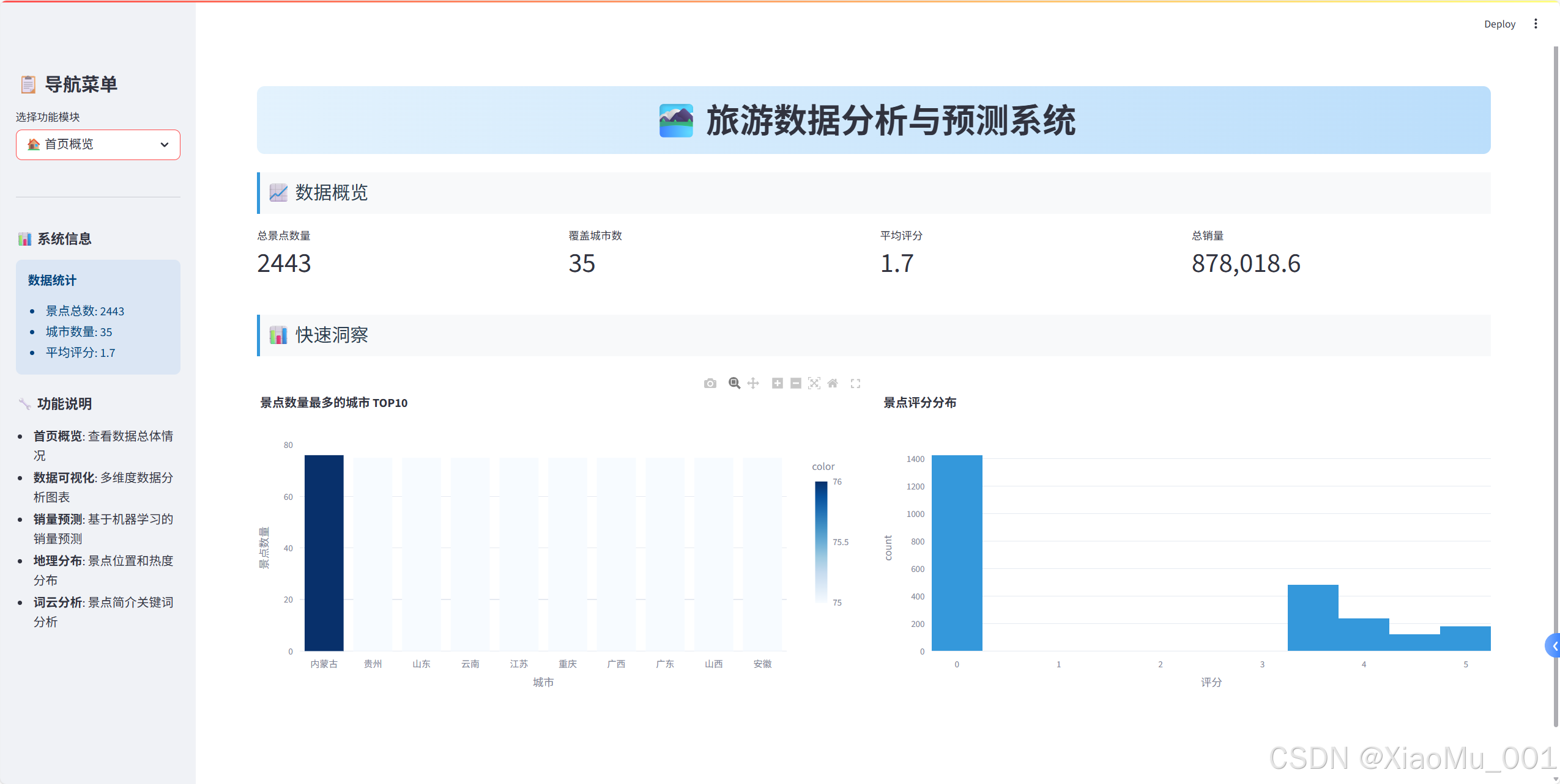
關鍵指標展示

# 創建四列布局顯示關鍵指標
col1, col2, col3, col4 = st.columns(4)with col1:st.metric("總景點數量", len(raw_data))
with col2:st.metric("覆蓋城市數", raw_data['城市'].nunique())
with col3:avg_rating = raw_data['評分'].mean()st.metric("平均評分", f"{avg_rating:.1f}")
with col4:total_sales = raw_data['銷量'].sum()st.metric("總銷量", f"{total_sales:,}")

快速洞察圖表

# 城市景點數量分布
city_counts = raw_data['城市'].value_counts().head(10)
fig_city = px.bar(x=city_counts.index, y=city_counts.values,title="景點數量最多的城市 TOP10",labels={'x': '城市', 'y': '景點數量'},color=city_counts.values,color_continuous_scale='Blues'
)
st.plotly_chart(fig_city, use_container_width=True)

2. 數據可視化模塊

數據大屏可視化

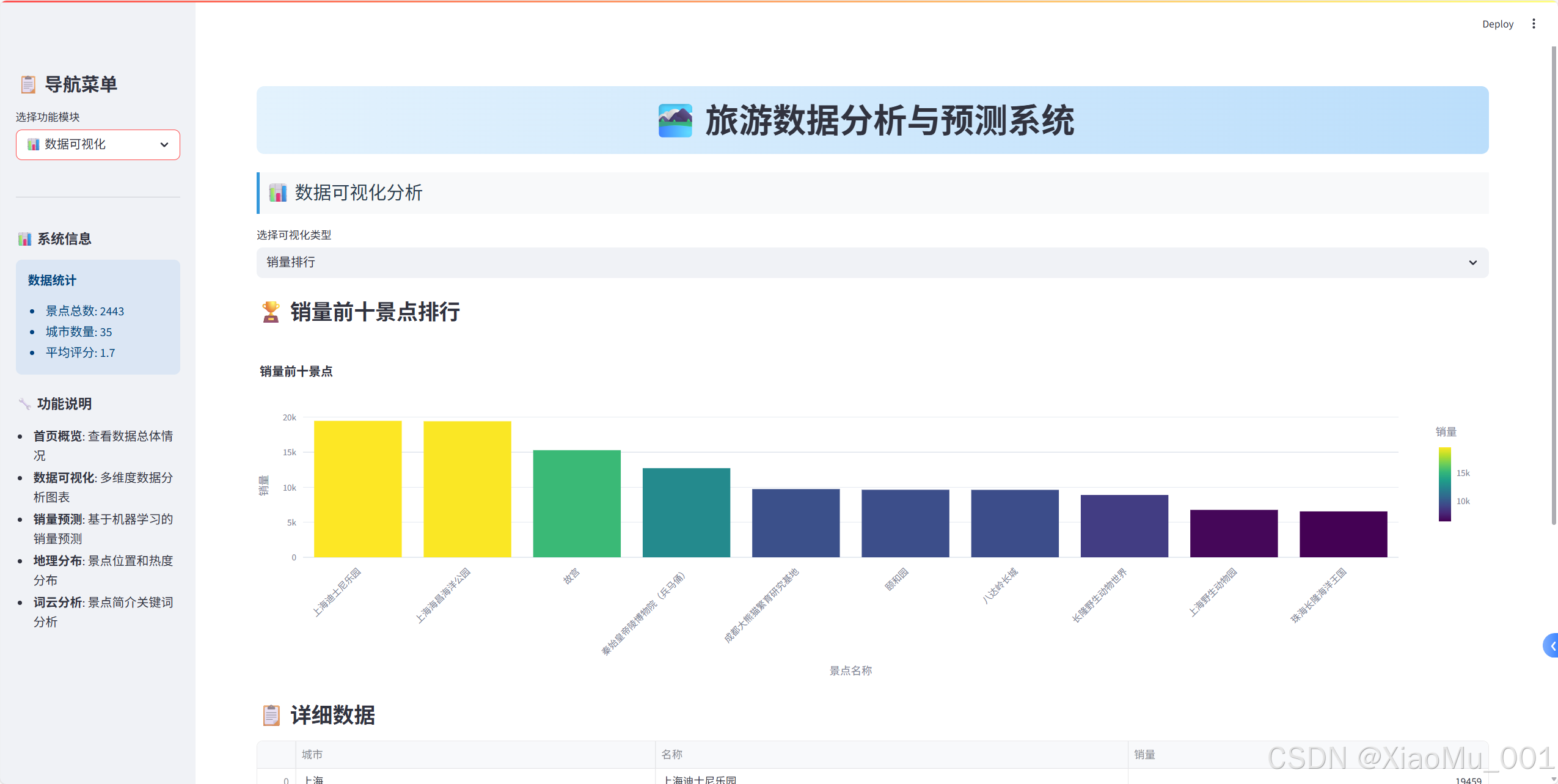
銷量排行分析

def create_sales_ranking():"""創建銷量排行圖表"""top_10_sales = raw_data[['城市', '名稱', '銷量']]\.sort_values(by='銷量', ascending=False).head(10)bar_chart = px.bar(top_10_sales, x='名稱', y='銷量',color='銷量',color_continuous_scale='Viridis',title="銷量前十景點",labels={'名稱': '景點名稱', '銷量': '銷量'})bar_chart.update_layout(xaxis_tickangle=-45)return bar_chart

星級分布分析

def create_star_distribution():"""創建星級分布圖表"""star_distribution = raw_data['星級'].value_counts().reset_index()star_distribution.columns = ['星級', '數量']# 餅圖pie_chart = px.pie(star_distribution, names='星級', values='數量',title="星級分布餅圖",color_discrete_sequence=px.colors.qualitative.Set3)# 柱狀圖bar_chart = px.bar(star_distribution,x='星級',y='數量',title="星級分布柱狀圖",color='數量',color_continuous_scale='Blues')return pie_chart, bar_chart

城市評分與價格關聯分析

def create_city_analysis():"""創建城市分析散點圖"""# 排除異常值df_no_sanqing = raw_data[raw_data['名稱'] != '三清山']# 計算城市平均值avg_score_price = df_no_sanqing.groupby('城市').agg({'評分': 'mean', '價格': 'mean'}).reset_index()avg_score_price = avg_score_price.sort_values(by='評分', ascending=False).head(10)scatter_chart = px.scatter(avg_score_price, x='評分', y='價格',color='城市',size='評分',size_max=20,title="平均評分前十城市與價格散點圖",labels={'評分': '平均評分', '價格': '平均價格（元）'},hover_data=['城市'])return scatter_chart

🔮 機器學習預測系統

預測模型設計

在這里插入圖片描述

1. 特征工程

def process_star(x):"""處理星級特征"""if 'A' in str(x):return int(str(x)[0])  # 提取數字部分else:return 0  # 無星級設為0

2. 數據預處理Pipeline

from sklearn.compose import ColumnTransformer
from sklearn.preprocessing import OneHotEncoder, StandardScaler# 創建預處理器
preprocessor = ColumnTransformer(transformers=[# 類別特征：獨熱編碼('cat', OneHotEncoder(handle_unknown='ignore'), ['城市', '名稱']),# 數值特征：標準化('num', StandardScaler(), ['星級', '評分'])])

3. 模型訓練Pipeline

from sklearn.pipeline import Pipeline
from sklearn.linear_model import LinearRegression# 創建完整的ML Pipeline
model = Pipeline(steps=[('preprocessor', preprocessor),('regressor', LinearRegression())
])# 特征和目標變量
X = df[['城市', '名稱', '星級', '評分', '是否免費']]
y = df['銷量']# 訓練模型
model.fit(X, y)

4. 預測接口實現

def predict_sales(city, spot_name, star_rating, rating, is_free):"""銷量預測函數"""# 構建輸入數據user_input = pd.DataFrame({'城市': [city],'名稱': [spot_name],'星級': [star_rating],'評分': [rating],'是否免費': [is_free]})# 進行預測predicted_sales = model.predict(user_input)return predicted_sales[0]

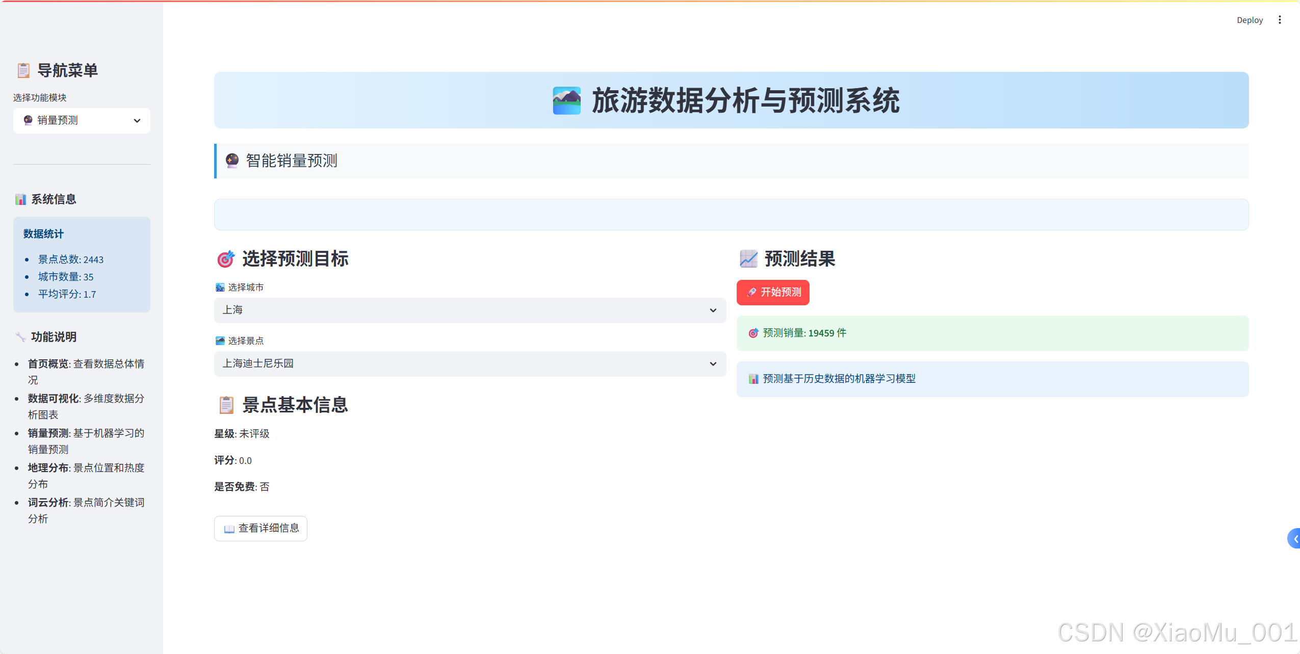
預測界面實現

def create_prediction_interface():"""創建預測界面"""with st.container():col1, col2 = st.columns(2)with col1:st.subheader("🎯 選擇預測目標")# 城市選擇cities = feature_data['城市'].unique()selected_city = st.selectbox('🏙? 選擇城市', cities)# 景點選擇city_spots = feature_data[feature_data['城市'] == selected_city]['名稱'].unique()selected_spot = st.selectbox('🏞? 選擇景點', city_spots)with col2:st.subheader("📈 預測結果")if st.button('🚀 開始預測', type='primary'):# 獲取景點信息spot_data = get_spot_data(selected_city, selected_spot)# 進行預測prediction = predict_sales(selected_city, selected_spot,spot_data['星級'], spot_data['評分'], spot_data['是否免費'])# 顯示結果st.success(f"🎯 預測銷量: **{prediction:.0f}** 件")

🗺? 地理數據可視化

在這里插入圖片描述

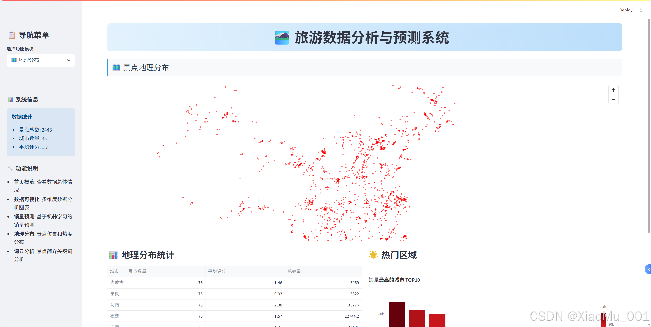
Pydeck地圖實現

1. 坐標數據處理

def process_coordinates(df):"""處理坐標數據"""# 分離經緯度df[['longitude', 'latitude']] = df['坐標'].str.split(',', expand=True)df['longitude'] = pd.to_numeric(df['longitude'], errors='coerce')df['latitude'] = pd.to_numeric(df['latitude'], errors='coerce')# 過濾無效坐標return df.dropna(subset=['longitude', 'latitude'])

2. 地圖視圖配置

import pydeck as pdk# 設置地圖視圖
view_state = pdk.ViewState(latitude=35.8617,   # 中國中心緯度longitude=104.1954, # 中國中心經度zoom=3,            # 縮放級別pitch=0,           # 俯仰角度
)

3. 散點圖層創建

# 創建散點圖層
layer = pdk.Layer("ScatterplotLayer",df_map,get_position=["longitude", "latitude"],get_radius=10000,              # 點的半徑get_color=[255, 0, 0, 160],    # 紅色半透明pickable=True,                 # 可點擊
)

4. 交互式地圖組裝

# 創建地圖對象
deck = pdk.Deck(layers=[layer],initial_view_state=view_state,tooltip={"text": "{名稱}\n城市: {城市}\n評分: {評分}\n銷量: {銷量}"},map_style="mapbox://styles/mapbox/light-v10"  # 淺色主題
)# 在Streamlit中顯示
st.pydeck_chart(deck, use_container_width=True)

地理統計分析

def create_geographic_stats(df_map):"""創建地理統計信息"""# 按城市統計region_stats = df_map.groupby('城市').agg({'名稱': 'count',     # 景點數量'評分': 'mean',      # 平均評分'銷量': 'sum'        # 總銷量}).round(2)region_stats.columns = ['景點數量', '平均評分', '總銷量']# 熱門區域分析hot_regions = df_map.groupby('城市')['銷量'].sum()\.sort_values(ascending=False).head(10)return region_stats, hot_regions

?? 文本數據挖掘

在這里插入圖片描述

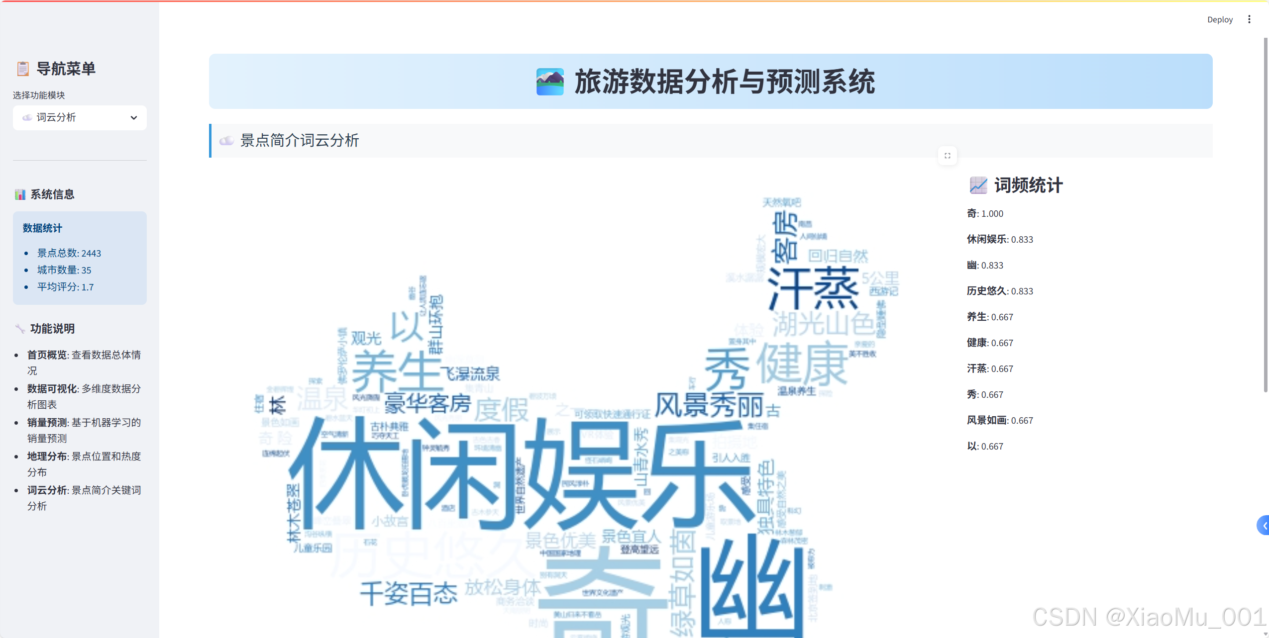
詞云生成實現

1. 文本預處理

def preprocess_text(descriptions):"""文本預處理"""# 合并所有簡介文本text = " ".join(descriptions.dropna().values)# 定義停用詞stopwords = set(["被譽為", "有", "之稱", "和", "是", "的", "在", "為", "一", "名", "景點", "素有", "餐飲", "中國", "世界", "最", "大", "多", "被", "包含", "這", "些", "該", "多個", "此", "風景", "之譽", "在這里", "旅游", "娛樂"])return text, stopwords

2. 詞云參數配置

def create_wordcloud_config(text, stopwords, mask=None):"""創建詞云配置"""config = {'width': 800,'height': 400,'max_words': 200,'max_font_size': 100,'contour_width': 1,'contour_color': 'white','colormap': 'Blues','background_color': 'white','font_path': "C:/Windows/Fonts/msyh.ttc",  # 中文字體'stopwords': stopwords}# 添加自定義形狀if mask is not None:config['mask'] = maskreturn config

3. 詞云生成與展示

def generate_and_display_wordcloud():"""生成并顯示詞云"""try:# 加載自定義形狀custom_mask = np.array(Image.open('map_copy.png'))mask_available = Trueexcept:mask_available = Falsest.warning("未找到自定義形狀文件，將使用默認形狀")# 生成詞云wordcloud_params = create_wordcloud_config(text, stopwords, custom_mask if mask_available else None)wordcloud = WordCloud(**wordcloud_params).generate(text)# 雙列布局展示col1, col2 = st.columns([3, 1])with col1:st.image(wordcloud.to_array(), use_container_width=True)with col2:st.subheader("📈 詞頻統計")word_freq = wordcloud.words_top_words = dict(list(word_freq.items())[:10])for word, freq in top_words.items():st.write(f"**{word}**: {freq:.3f}")

替代方案：詞頻統計圖表

def create_word_frequency_chart(text, stopwords):"""創建詞頻統計圖表（WordCloud不可用時的替代方案）"""from collections import Counter# 簡單分詞和過濾words = text.split()filtered_words = [word for word in words if word not in stopwords and len(word) > 1]# 統計詞頻word_counts = Counter(filtered_words).most_common(20)# 創建DataFramewords_df = pd.DataFrame(word_counts, columns=['詞語', '頻次'])# 創建柱狀圖fig = px.bar(words_df, x='詞語', y='頻次',title="關鍵詞頻率統計 TOP20",color='頻次',color_continuous_scale='Blues')fig.update_layout(xaxis_tickangle=-45)return fig, words_df

? 性能優化策略

1. 數據緩存機制

@st.cache_data
def load_data():"""緩存數據加載"""raw_data = pd.read_csv('tourism_raw_data.csv')feature_data = pd.read_csv('tourism_feature_data.csv')return raw_data, feature_data@st.cache_resource
def train_model(feature_data):"""緩存模型訓練"""# 模型訓練代碼# ...return model

緩存策略說明：

@st.cache_data：用于緩存數據加載操作
@st.cache_resource：用于緩存資源密集型操作（如模型訓練）
避免重復計算，顯著提升應用響應速度

2. 條件導入處理

# 優雅處理可選依賴
try:from wordcloud import WordCloudWORDCLOUD_AVAILABLE = True
except ImportError:WORDCLOUD_AVAILABLE = Falsest.warning("WordCloud 庫未安裝，詞云功能將不可用。")

3. 異步加載策略

def lazy_load_components():"""延遲加載組件"""if 'model_trained' not in st.session_state:with st.spinner('正在訓練模型...'):st.session_state.model_trained = train_model(feature_data)return st.session_state.model_trained

🔧 容錯處理與用戶體驗

1. 錯誤處理機制

def safe_execute(func, error_msg="操作失敗"):"""安全執行函數"""try:return func()except Exception as e:st.error(f"{error_msg}: {str(e)}")return None

2. 用戶反饋系統

def show_loading_progress():"""顯示加載進度"""progress_bar = st.progress(0)status_text = st.empty()for i in range(100):progress_bar.progress(i + 1)status_text.text(f'加載中... {i+1}%')time.sleep(0.01)status_text.text('加載完成！')

3. 響應式設計

def create_responsive_layout():"""創建響應式布局"""# 根據屏幕寬度調整列數if st.session_state.get('mobile_view', False):col1, col2 = st.columns(1), st.columns(1)else:col1, col2 = st.columns(2)

📦 部署與配置

1. 依賴管理

# requirements.txt
streamlit
pandas
numpy
plotly
pydeck
matplotlib
scikit-learn
Pillow
wordcloud
collections-extended

2. 啟動腳本

#!/bin/bash
# run_app.sh
echo "啟動旅游數據分析系統..."
streamlit run streamlit_integrated_app.py --server.port 8501

3. Docker部署（可選）

FROM python:3.9-slimWORKDIR /app
COPY requirements.txt .
RUN pip install -r requirements.txtCOPY . .
EXPOSE 8501CMD ["streamlit", "run", "streamlit_integrated_app.py"]

🚀 項目運行指南

環境準備

# 1. 克隆項目
git clone <repository-url>
cd tourism-analysis-system# 2. 安裝依賴
pip install -r requirements.txt# 3. 準備數據文件
# 確保以下文件存在：
# - tourism_raw_data.csv
# - tourism_feature_data.csv
# - map_copy.png (可選)# 4. 啟動應用
streamlit run streamlit_integrated_app.py