人工智能概述
人工智能分為:符號學習,機器學習。
機器學習是實現人工智能的一種方法,深度學習是實現機器學習的一種技術。
機器學習:使用算法來解析數據,從中學習,然后對真實世界中是事務進行決策和預測。如垃圾郵件檢測,樓房價格預測。
深度學習:模仿人類神經網絡,建立模型,進行數據分析。如,人臉識別,語義理解,無人駕駛。
工具
Anaconda
Anaconda是一個方便的python包管理和環境管理的軟件
可以跨平臺,多python版本并存,部署方便
Jupyter Notebook
Jupyter notebook是一個開源的web應用程序,允許開發者方便的創建和共享代碼文檔
允許吧代碼寫入獨立的cell中,單獨執行。用戶可以單獨測試特定代碼塊,無需從頭開始執行代碼。
基礎工具包
Panda
強大的分析結構化數據的工具集,可用于快速實現數據導入/出,索引
www.pypandas.cn
Numpy
使用Python進行科學計算的基礎軟件包。核心:基于N維數組對象ndarray的數組運算。
www.numpy.org.cn
Matplolib
Python基礎繪圖庫,幾行代碼即可生成繪圖
www.matplotlib.org.cn
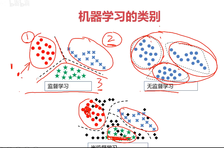
機器學習的類別
監督學習(Supervised Learning)
-訓練數據包括正確的結果
無監督學習(Unsupervised Learning)
-訓練數據不包括正確的結果
半監督學習(Semi-supervised Learning)
-訓練數據包括少量正確的結果
強化學習(Reinforcement Learning)
-根據每次結果收獲的獎懲進行學習,實現優化
監督學習:線性回歸,邏輯回歸,決策樹,神經網絡,卷積神經網絡,循環神經網絡。
無監督學習:聚類算法
混合學習:監督學習+無監督學習
什么是回歸分析?
回歸分析:根據數據,確定兩種或兩種以上變量間相互依賴的定量關系
線性回歸:回歸分析中,變量與因變量存在線性關系
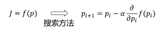
梯度下降法:
尋找極小值的一種方法。通過向函數上當前點對應梯度的反方向的規定步長距離點進行迭代搜索,直到在極小點收斂。
Scikit-learn
Python語言中專門針對機器學習應用而發展起來的一款開源框架(算法庫),可以實現數據預處理,分類,回歸,降維,模型選擇等常用的機器學習算法
集成了機器學習中各類成熟的算法,不支持深度學習和強化學習。
https://scikit-learn.org/stable/index.html
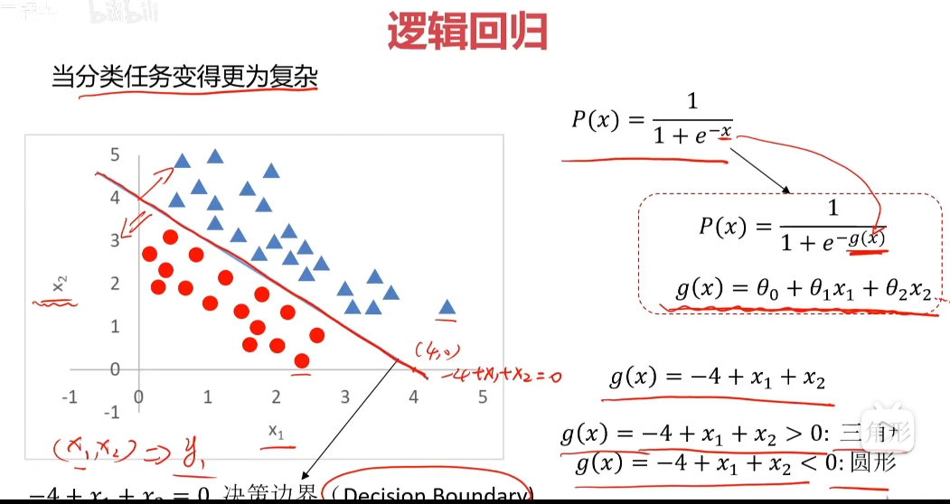
分類問題
分類:根據已知樣本的某些特征,判斷一個顯得樣本屬于那種已知的樣本類
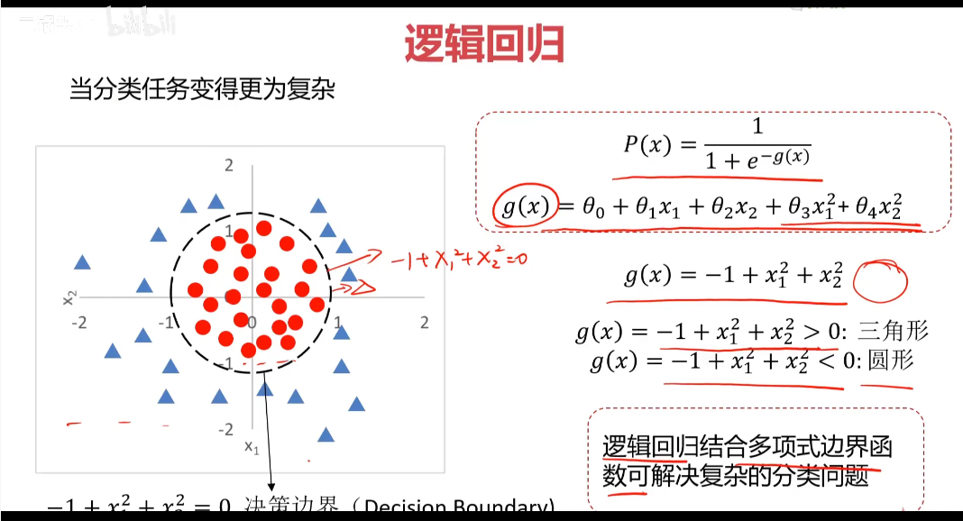
使用邏輯回歸擬合數據,可以很好的完成分類任務
線性:y=ax+b
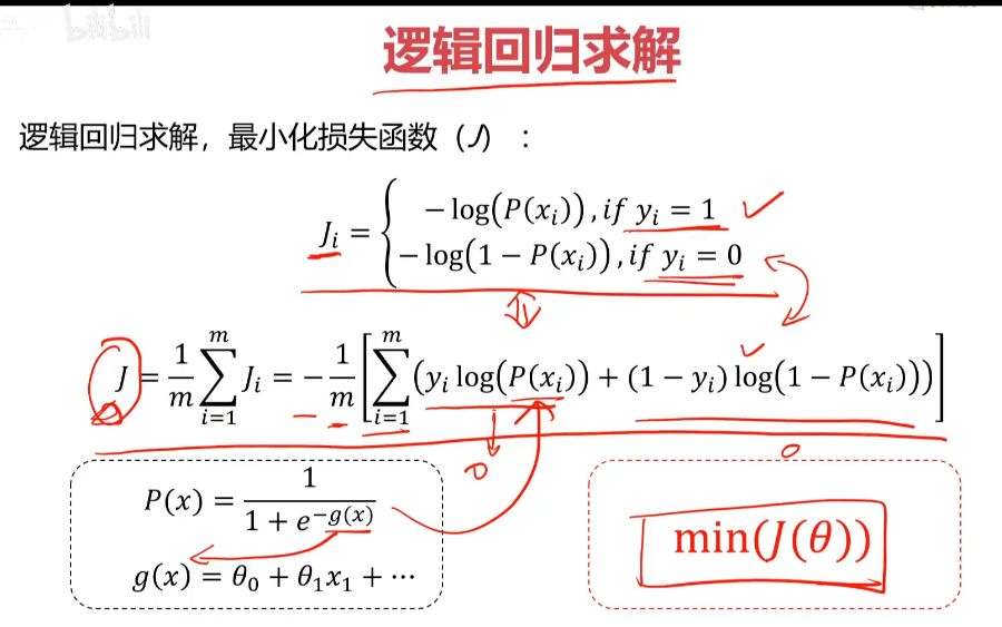
邏輯:y=1/(1+e^(-x)) sigmoid方程 通用公式:P(x)=1/(1+e^(-g(x)))
找到決策邊界(Decision Boundary)很關鍵
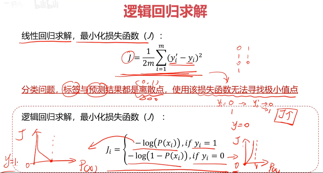
分類任務的損失函數:
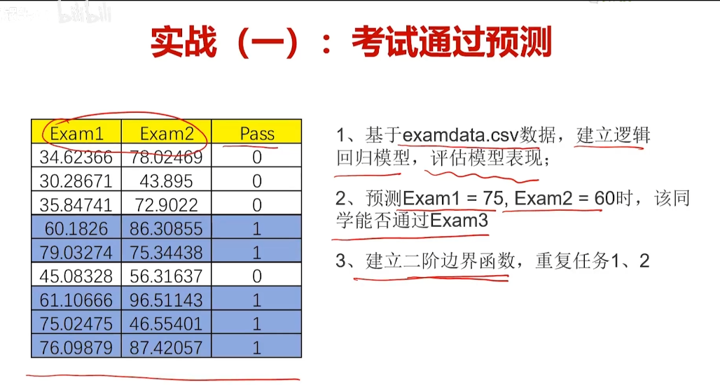
邏輯回歸實戰
實戰1考試通過預測
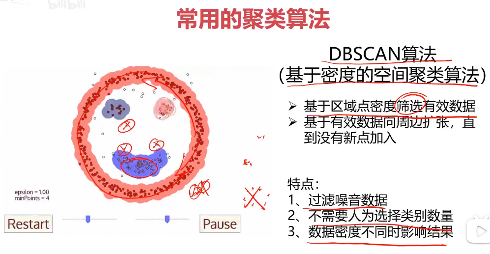
無監督學習
機器學習的一種方法,沒有給定先標記過的訓練示例,自動對輸入的數據進行分類或分群
聚類分析
聚類分析又稱為群分析,根據對象某些屬性的相似度,將其自動劃分為不同的類別。
應用場景:客戶劃分,基因聚類,新聞關聯
KMeans
K-均值算法:以空間中k個點為中心進行聚類,對最靠近他們的對象歸類,是聚類算法中最為基礎但也最為重要的算法。
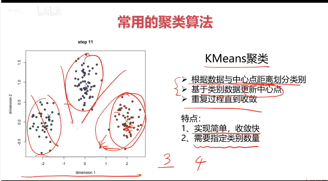
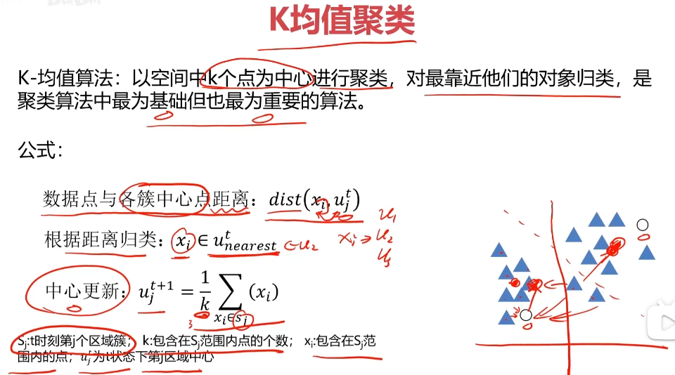
算法流程:
1.選擇聚類的個數k
2.確定聚類的中心
3.根據點道聚類中心聚類確定各個點所屬類別
4.根據各個類別數據更新聚類中心
5.重復以上步驟直到收斂(中心點不再變化)
優點:
1.簡單易實現,收斂速度快
2.參數少
缺點:
1.必須設置簇的數量
2.隨機選擇初始聚類中心,結果可能缺乏一致性
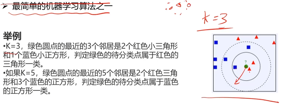
KNN
K近鄰分類模型
給定一個訓練數據集,對新的輸入實例,在訓練數據集中找到與該實例最鄰近的K個實例(也就是上面所說的K個鄰居),這K個實例的多數屬于某個類,就把該輸入實例分類到這個類中
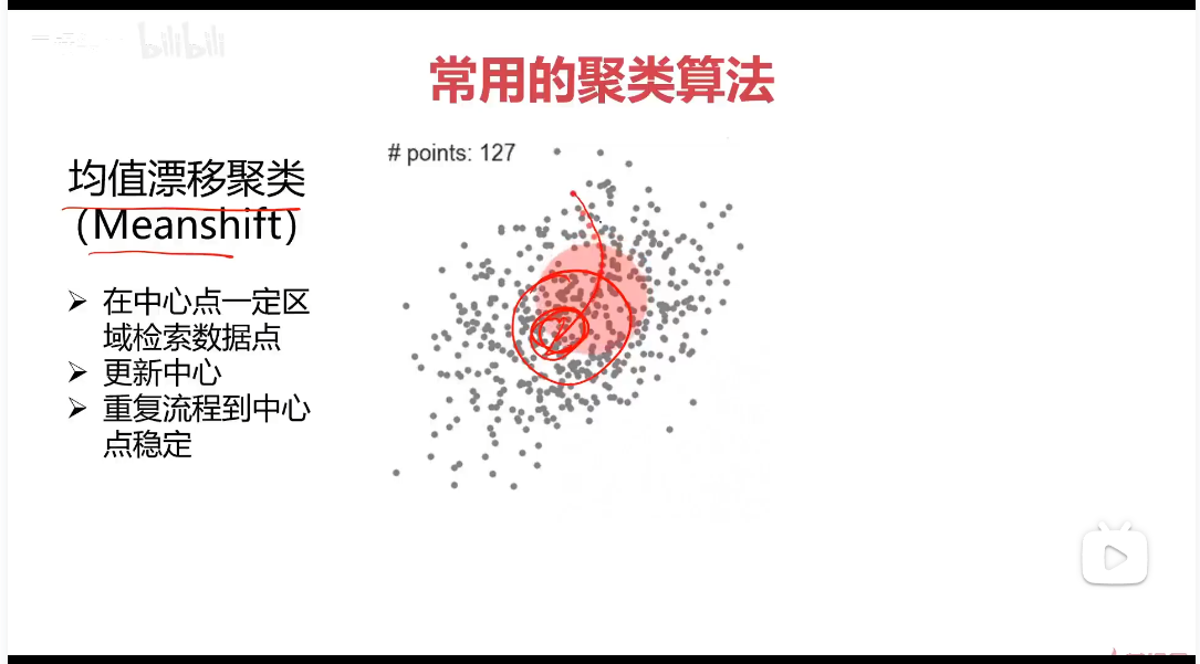
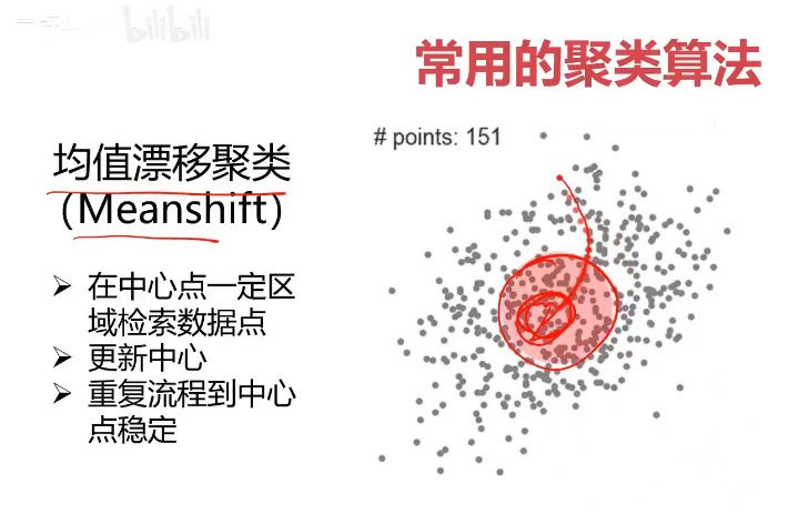
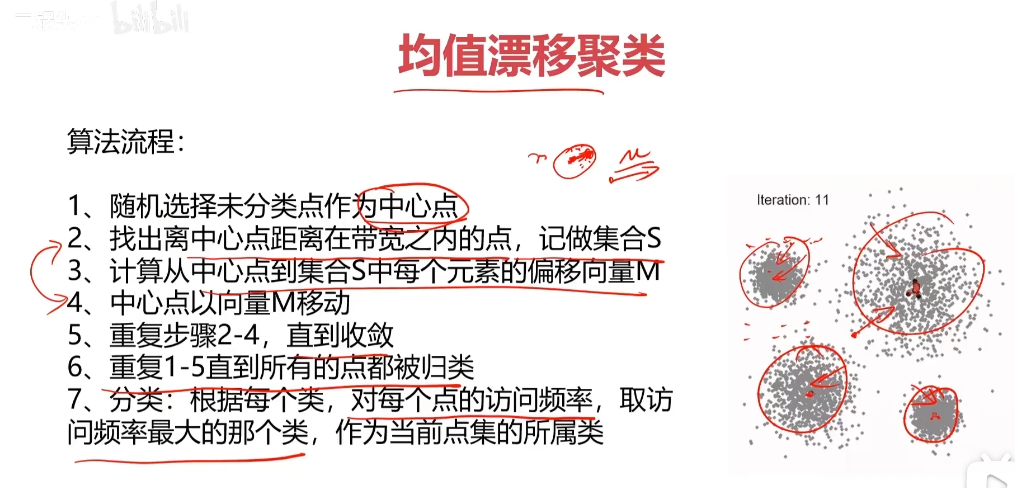
Mean-shift
聚類實戰
KMeans實現聚類
模型訓練
form sklearn.cluster import KMeans
KM = KMeans(n_clusters=3,random_state=0)
KM.fit(X)
獲取中心點:
centers = KM.cluster_centers_
準確率計算:
form sklearn.metrics import accuracy_score
accuracy = accuracy_score(y,y_predict)
預測結果矯正(比如原始數據是0,1,2但是KNN預測的亂序了,如2,0,1):
y_cal = []
for i in y_predict:if i == 0:y_cla.append(2)elif i == 1:y_cal.append(0)else:y_cal.append(1)print(y_predict, y_cal0
Meanshift實現聚類
自動計算帶寬(區域半徑)
from sklearn.cluster import MeanShift,estimate_bandwidth
#detect bandwidth
bandwidth = estimate_bandwidth(X,n_samples=500)
#X樣本數量,n_samples采樣的樣本數量
模型建立于訓練
ms = MeanShift(bandwidth=bandwidth)
ms.fit(X)
KNN實現分類
模型訓練
form sklearn.neighbors import KNeighborsClassifier
KNN = KNeighborsClassifier(n_neighbors=3)
KNN.fit(X,y)
實戰:2D數據類別劃分
1.采用Kmeans算法實現2D數據自動聚類,預測V1=80,V2=60數據類別;
2.計算預測準確率,完成結果矯正
3.采用KNN,Meanshift算法,重復步驟1-2
KMeans算法實現
#load the data
import pandas as pd
import numpy as np
data = pd.read_csv('data.csv')
data.head()
#define X and y
X = data.drop(['labels'],axis=1)
y = data.loc[:,'labels']
y.head()
pd.value_counts(y)
%matplotlib inline
from matplotlib import pyplot as plt
plt.scatter(X.loc[:,'V1'],X.loc[:'V2'])
plt.title("un-labled data")
plt.xlabel('V1')
plt.ylabel('V2')
plt.show()fig1 = plt.figure()
label0 = plt.scatter(X.loc[:,'V1'][y==0],X.loc[:'V2'][y==0])
label1 = plt.scatter(X.loc[:,'V1'][y==1],X.loc[:'V2'][y==1])
label2 = plt.scatter(X.loc[:,'V1'][y==2],X.loc[:'V2'][y==2])plt.title("labled data")
plt.xlabel('V1')
plt.ylabel('V2')
plt.legend((label0,label1,label2),('label0','label1','label2'))
plt.show()
print(X.shape, y.shape)
#set the model
from sklearn.cluster import KMeans
KM = KMeans(n_cluster=3,random_sate=0)
KM.fit(X)centers = KM.cluster_centers_
fig3 = plt.figure()
label0 = plt.scatter(X.loc[:,'V1'][y==0],X.loc[:'V2'][y==0])
label1 = plt.scatter(X.loc[:,'V1'][y==1],X.loc[:'V2'][y==1])
label2 = plt.scatter(X.loc[:,'V1'][y==2],X.loc[:'V2'][y==2])plt.title("labled data")
plt.xlabel('V1')
plt.ylabel('V2')
plt.legend((label0,label1,label2),('label0','label1','label2'))
plt.scatter(centers[:,0],centers[:,1])
plt.show()
#test data: V1=80,V2=60
y_predict_test = KM.predict([[80, 60]])
print(y_predict_test )#predict based on training data
y_predict = KM.predict(X)
print(pd.value_counts(y_predict), pd.value_counts(y))from sklearn.metrics import accuracy_score
accuracy = accuracy_score(y,y_predict)
print(accuracy)
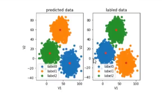
#visualize the data and results
fig4 = plt.subplot(121)
label0 = plt.scatter(X.loc[:,'V1'][y_predict==0],X.loc[:'V2'][y_predict==0])
label1 = plt.scatter(X.loc[:,'V1'][y_predict==1],X.loc[:'V2'][y_predict==1])
label2 = plt.scatter(X.loc[:,'V1'][y_predict==2],X.loc[:'V2'][y_predict==2])plt.title("predict data")
plt.xlabel('V1')
plt.ylabel('V2')
plt.legend((label0,label1,label2),('label0','label1','label2'))
plt.scatter(centers[:,0],centers[:,1])fig5 = plt.subplot(122)
label0 = plt.scatter(X.loc[:,'V1'][y==0],X.loc[:'V2'][y==0])
label1 = plt.scatter(X.loc[:,'V1'][y==1],X.loc[:'V2'][y==1])
label2 = plt.scatter(X.loc[:,'V1'][y==2],X.loc[:'V2'][y==2])plt.title("labled data")
plt.xlabel('V1')
plt.ylabel('V2')
plt.legend((label0,label1,label2),('label0','label1','label2'))
plt.scatter(centers[:,0],centers[:,1])plt.show()
#correct the resultsy_corrected = []for i in y_predict:if i == 0:y_corrected.append(1)elif i == 1:y_corrected.append(2) else:y_corrected.append(0) print(pd.value_counts(y_corrected), pd.value_counts(y))
print(accuracy_score(y, y_corrected))
y_corrected = np.array(y_corrected)
print(type(y_corrected))
#visualize the data and results
fig6 = plt.subplot(121)
label0 = plt.scatter(X.loc[:,'V1'][y_corrected==0],X.loc[:'V2'][y_corrected==0])
label1 = plt.scatter(X.loc[:,'V1'][y_corrected==1],X.loc[:'V2'][y_corrected==1])
label2 = plt.scatter(X.loc[:,'V1'][y_corrected==2],X.loc[:'V2'][y_corrected==2])plt.title("predict data")
plt.xlabel('V1')
plt.ylabel('V2')
plt.legend((label0,label1,label2),('label0','label1','label2'))
plt.scatter(centers[:,0],centers[:,1])fig7 = plt.subplot(122)
label0 = plt.scatter(X.loc[:,'V1'][y==0],X.loc[:'V2'][y==0])
label1 = plt.scatter(X.loc[:,'V1'][y==1],X.loc[:'V2'][y==1])
label2 = plt.scatter(X.loc[:,'V1'][y==2],X.loc[:'V2'][y==2])plt.title("labled data")
plt.xlabel('V1')
plt.ylabel('V2')
plt.legend((label0,label1,label2),('label0','label1','label2'))
plt.scatter(centers[:,0],centers[:,1])plt.show()
KNN算法實現
查看數據
X.head()
y.head()
#establish a KNN model
from sklearn.neighbors import KNeighborsClassifier
KNN = KNeighborsClassifier(n_neighbors=3)
KNN.fit(X,y)
#predict based on the test data V1=80, V2=60
y_predict_knn_test = KNN.predict([[80, 60]])
y_predict_knn = KNN.predict(X)
print(y_predict_knn_test)
print('knn accuracy:', accuracy_score(y, y_predict_knn))
fig6 = plt.subplot(121)
label0 = plt.scatter(X.loc[:,'V1'][y_predict_knn==0],X.loc[:'V2'][y_predict_knn==0])
label1 = plt.scatter(X.loc[:,'V1'][y_predict_knn==1],X.loc[:'V2'][y_predict_knn==1])
label2 = plt.scatter(X.loc[:,'V1'][y_predict_knn==2],X.loc[:'V2'][y_predict_knn==2])plt.title("knn results")
plt.xlabel('V1')
plt.ylabel('V2')
plt.legend((label0,label1,label2),('label0','label1','label2'))
plt.scatter(centers[:,0],centers[:,1])fig7 = plt.subplot(122)
label0 = plt.scatter(X.loc[:,'V1'][y==0],X.loc[:'V2'][y==0])
label1 = plt.scatter(X.loc[:,'V1'][y==1],X.loc[:'V2'][y==1])
label2 = plt.scatter(X.loc[:,'V1'][y==2],X.loc[:'V2'][y==2])plt.title("labled data")
plt.xlabel('V1')
plt.ylabel('V2')
plt.legend((label0,label1,label2),('label0','label1','label2'))
plt.scatter(centers[:,0],centers[:,1])plt.show()
MeanShift
#meanshift
form sklearn.cluster import MeanShift,estimate_bandwidth
#obtain the bandwidth
bw = estimate_bandwidth(X,n_samples=500)
print(bw)
#establish the meanshift model-un-supervised model
ms = MeanShift(bandwidth=bw)
ms.fit(X)
y_predict_ms = ms.predict(X)
print(pd.value_counts(y_predict_ms), pd.value_counts(y))
fig6 = plt.subplot(121)
label0 = plt.scatter(X.loc[:,'V1'][y_predict_knn_ms==0],X.loc[:'V2'][y_predict_knn_ms==0])
label1 = plt.scatter(X.loc[:,'V1'][y_predict_knn_ms==1],X.loc[:'V2'][y_predict_knn_ms==1])
label2 = plt.scatter(X.loc[:,'V1'][y_predict_knn_ms==2],X.loc[:'V2'][y_predict_knn_ms==2])plt.title("kmeanshift results")
plt.xlabel('V1')
plt.ylabel('V2')
plt.legend((label0,label1,label2),('label0','label1','label2'))
plt.scatter(centers[:,0],centers[:,1])fig7 = plt.subplot(122)
label0 = plt.scatter(X.loc[:,'V1'][y==0],X.loc[:'V2'][y==0])
label1 = plt.scatter(X.loc[:,'V1'][y==1],X.loc[:'V2'][y==1])
label2 = plt.scatter(X.loc[:,'V1'][y==2],X.loc[:'V2'][y==2])plt.title("labled data")
plt.xlabel('V1')
plt.ylabel('V2')
plt.legend((label0,label1,label2),('label0','label1','label2'))
plt.scatter(centers[:,0],centers[:,1])plt.show()
#correct the resultsy_corrected_ms = []for i in y_predict_ms:if i == 0:y_corrected_ms .append(2)elif i == 1:y_corrected_ms .append(1) else:y_corrected_ms .append(0) print(pd.value_counts(y_corrected_ms), pd.value_counts(y))
#convert the results to numpy array
y_corrected = np.array(y_corrected_ms)
print(type(y_corrected_ms)
fig6 = plt.subplot(121)
label0 = plt.scatter(X.loc[:,'V1'][y_predict_knn_ms==0],X.loc[:'V2'][y_predict_knn_ms==0])
label1 = plt.scatter(X.loc[:,'V1'][y_predict_knn_ms==1],X.loc[:'V2'][y_predict_knn_ms==1])
label2 = plt.scatter(X.loc[:,'V1'][y_predict_knn_ms==2],X.loc[:'V2'][y_predict_knn_ms==2])plt.title("ms correct results")
plt.xlabel('V1')
plt.ylabel('V2')
plt.legend((label0,label1,label2),('label0','label1','label2'))
plt.scatter(centers[:,0],centers[:,1])fig7 = plt.subplot(122)
label0 = plt.scatter(X.loc[:,'V1'][y==0],X.loc[:'V2'][y==0])
label1 = plt.scatter(X.loc[:,'V1'][y==1],X.loc[:'V2'][y==1])
label2 = plt.scatter(X.loc[:,'V1'][y==2],X.loc[:'V2'][y==2])plt.title("labled data")
plt.xlabel('V1')
plt.ylabel('V2')
plt.legend((label0,label1,label2),('label0','label1','label2'))
plt.scatter(centers[:,0],centers[:,1])
plt.show()
##總結
kmeans\knn\meanshift
kmeans\meanshift: un-supervised, training data: X; kmeans: category number; meanshift: calculate the bandwidth
knn: supervised; training data: X\y
——DDS信號發生器設計)

)


 (傳輸協議層:UDP、TCP))


——ViT理解與應用)


