目標

在本實驗中，你將:使用梯度下降自動化優化w和b的過程

工具

在本實驗中，我們將使用:

• NumPy，一個流行的科學計算庫
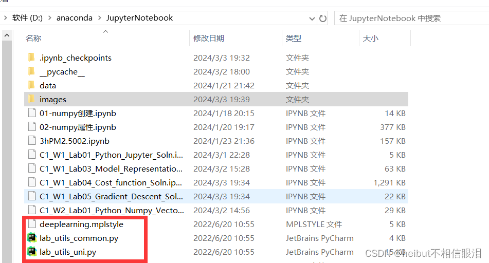
• Matplotlib，一個用于繪制數據的流行庫在本地目錄的
• lab_utils.py文件中繪制例程

import math, copy
import numpy as np
import matplotlib.pyplot as plt
plt.style.use('./deeplearning.mplstyle')
from lab_utils_uni import plt_house_x, plt_contour_wgrad, plt_divergence, plt_gradients

當前jupyter note工作目錄需要包含：

問題陳述

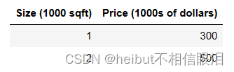
讓我們使用和之前一樣的兩個數據點——一個1000平方英尺的房子賣了30萬美元，一個2000平方英尺的房子賣了50萬美元。

# Load our data set
x_train = np.array([1.0, 2.0])   #features
y_train = np.array([300.0, 500.0])   #target value

計算損失

這是上一個實驗室開發的。我們這里還會用到它

#Function to calculate the cost
def compute_cost(x, y, w, b):m = x.shape[0] cost = 0for i in range(m):f_wb = w * x[i] + bcost = cost + (f_wb - y[i])**2total_cost = 1 / (2 * m) * costreturn total_cost

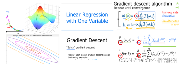
梯度下降總結

線性模型：f（x）=wx+b
損失函數：J（w，b）

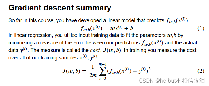
參數更新：

執行梯度下降

def compute_gradient(x, y, w, b): """Computes the gradient for linear regression Args:x (ndarray (m,)): Data, m examples y (ndarray (m,)): target valuesw,b (scalar)    : model parameters  Returnsdj_dw (scalar): The gradient of the cost w.r.t. the parameters wdj_db (scalar): The gradient of the cost w.r.t. the parameter b     """# Number of training examplesm = x.shape[0]    dj_dw = 0dj_db = 0for i in range(m):  f_wb = w * x[i] + b dj_dw_i = (f_wb - y[i]) * x[i] dj_db_i = f_wb - y[i] dj_db += dj_db_idj_dw += dj_dw_i dj_dw = dj_dw / m dj_db = dj_db / m return dj_dw, dj_db

plt_gradients(x_train,y_train, compute_cost, compute_gradient)
plt.show()

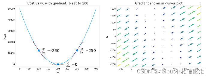
上面的左邊的圖固定了b=100。左圖顯示了成本曲線在三個點上相對于w的斜率。在圖的右邊，導數是正的，而在左邊，導數是負的。由于“碗形”，導數將始終導致梯度下降到梯度為零的底部。
梯度下降將利用損失函數對w和對b求偏導來更新參數。右側的“顫抖圖”提供了一種查看兩個參數梯度的方法。箭頭大小反映了該點的梯度大小。箭頭的方向和斜率反映了的比例在這一點上。注意，梯度點遠離最小值。從w或b的當前值中減去縮放后的梯度。這將使參數朝著降低成本的方向移動。

梯度下降法

既然可以計算梯度，那么上面式(3)中描述的梯度下降可以在下面的gradient_descent中實現。在評論中描述了實現的細節。下面，你將利用這個函數在訓練數據上找到w和b的最優值。

def gradient_descent(x, y, w_in, b_in, alpha, num_iters, cost_function, gradient_function): """Performs gradient descent to fit w,b. Updates w,b by taking num_iters gradient steps with learning rate alphaArgs:x (ndarray (m,))  : Data, m examples y (ndarray (m,))  : target valuesw_in,b_in (scalar): initial values of model parameters  alpha (float):     Learning ratenum_iters (int):   number of iterations to run gradient descentcost_function:     function to call to produce costgradient_function: function to call to produce gradientReturns:w (scalar): Updated value of parameter after running gradient descentb (scalar): Updated value of parameter after running gradient descentJ_history (List): History of cost valuesp_history (list): History of parameters [w,b] """w = copy.deepcopy(w_in) # avoid modifying global w_in# An array to store cost J and w's at each iteration primarily for graphing laterJ_history = []p_history = []b = b_inw = w_infor i in range(num_iters):# Calculate the gradient and update the parameters using gradient_functiondj_dw, dj_db = gradient_function(x, y, w , b)     # Update Parameters using equation (3) aboveb = b - alpha * dj_db                            w = w - alpha * dj_dw                            # Save cost J at each iterationif i<100000:      # prevent resource exhaustion J_history.append( cost_function(x, y, w , b))p_history.append([w,b])# Print cost every at intervals 10 times or as many iterations if < 10if i% math.ceil(num_iters/10) == 0:print(f"Iteration {i:4}: Cost {J_history[-1]:0.2e} ",f"dj_dw: {dj_dw: 0.3e}, dj_db: {dj_db: 0.3e}  ",f"w: {w: 0.3e}, b:{b: 0.5e}")return w, b, J_history, p_history #return w and J,w history for graphing

# initialize parameters
w_init = 0
b_init = 0
# some gradient descent settings
iterations = 10000
tmp_alpha = 1.0e-2
# run gradient descent
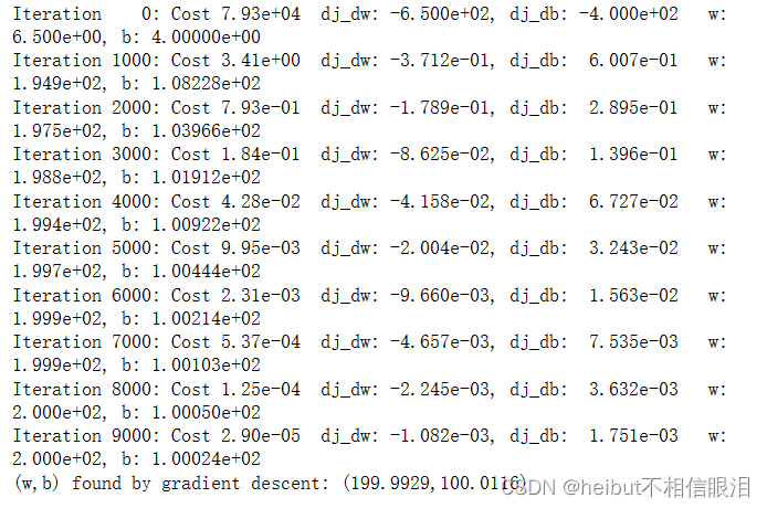
w_final, b_final, J_hist, p_hist = gradient_descent(x_train ,y_train, w_init, b_init, tmp_alpha, iterations, compute_cost, compute_gradient)
print(f"(w,b) found by gradient descent: ({w_final:8.4f},{b_final:8.4f})")

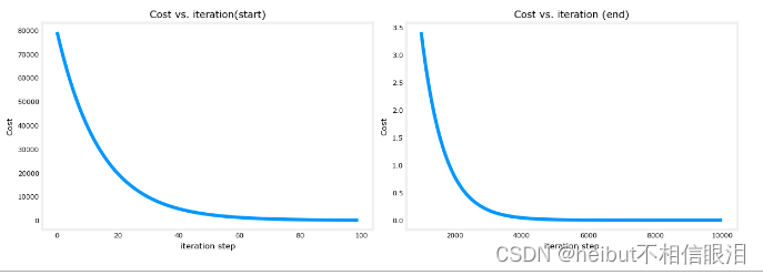
成本與梯度下降的迭代

代價與迭代的關系圖是衡量梯度下降過程的有用方法。在成功的運行中，成本應該總是降低的。最初成本的變化是如此之快，用不同的尺度來繪制最初的坡度和最終的下降是很有用的。在下面的圖表中，請注意軸上的成本比例和迭代步驟。

# plot cost versus iteration  
fig, (ax1, ax2) = plt.subplots(1, 2, constrained_layout=True, figsize=(12,4))
ax1.plot(J_hist[:100])
ax2.plot(1000 + np.arange(len(J_hist[1000:])), J_hist[1000:])
ax1.set_title("Cost vs. iteration(start)");  ax2.set_title("Cost vs. iteration (end)")
ax1.set_ylabel('Cost')            ;  ax2.set_ylabel('Cost') 
ax1.set_xlabel('iteration step')  ;  ax2.set_xlabel('iteration step') 
plt.show()

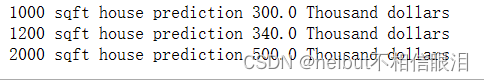
預測

現在您已經發現了參數w和b的最優值，您可以現在用這個模型根據我們學到的參數來預測房價。作為預期，預測值與訓練值幾乎相同住房。此外，不在預測中的值與期望值一致。

print(f"1000 sqft house prediction {w_final*1.0 + b_final:0.1f} Thousand dollars")
print(f"1200 sqft house prediction {w_final*1.2 + b_final:0.1f} Thousand dollars")
print(f"2000 sqft house prediction {w_final*2.0 + b_final:0.1f} Thousand dollars")

繪制

您可以通過在代價(w,b)的等高線圖上繪制迭代代價來顯示梯度下降的執行過程。

fig, ax = plt.subplots(1,1, figsize=(12, 6))
plt_contour_wgrad(x_train, y_train, p_hist, ax)

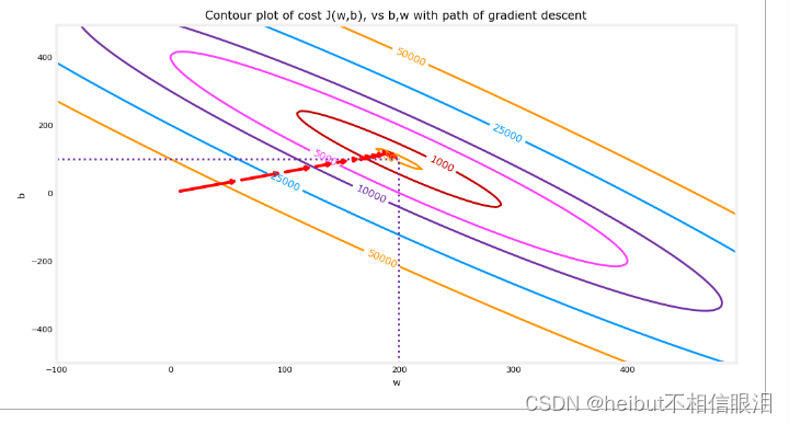
上圖等高線圖顯示了w和b范圍內的成本(w, b)用圓環表示。用紅色箭頭覆蓋的是梯度下降的路徑。以下是一些需要注意的事項:這條路平穩地(單調地)向目標前進。最初的步驟比接近目標的步驟要大得多。
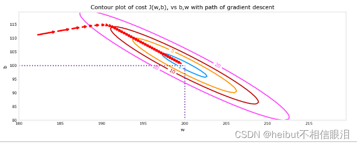
放大后，我們可以看到梯度下降的最后步驟。注意，當梯度趨于零時，步驟之間的距離會縮小。

fig, ax = plt.subplots(1,1, figsize=(12, 4))
plt_contour_wgrad(x_train, y_train, p_hist, ax, w_range=[180, 220, 0.5], b_range=[80, 120, 0.5],contours=[1,5,10,20],resolution=0.5)

# initialize parameters
w_init = 0
b_init = 0
# set alpha to a large value
iterations = 10
tmp_alpha = 8.0e-1
# run gradient descent
w_final, b_final, J_hist, p_hist = gradient_descent(x_train ,y_train, w_init, b_init, tmp_alpha, iterations, compute_cost, compute_gradient)

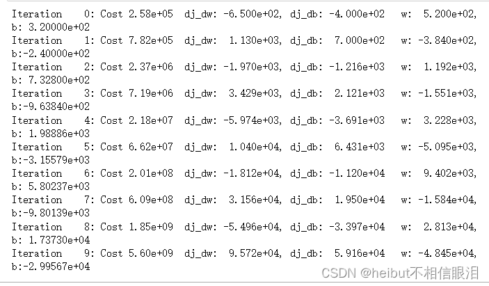
上面，w和b在正負之間來回跳躍，絕對值隨著每次迭代而增加。此外，每次迭代J(w,b)都會改變符號，成本也在增加W而不是遞減。這是一個明顯的跡象，表明學習率太大，解決方案是發散的。我們用一個圖來形象化。

plt_divergence(p_hist, J_hist,x_train, y_train)
plt.show()

上面，左圖顯示了w在梯度下降的前幾個步驟中的進展。W從正到負振蕩，成本迅速增長。梯度下降同時在兩個魔杖b上運行，因此需要右邊的3-D圖來獲得完整的圖像。

祝賀

在這個實驗中深入研究了單個變量的梯度下降的細節。開發了一個程序來計算梯度想象一下梯度是什么完成一個梯度下降程序利用梯度下降法求參數考察了確定學習率大小的影響