文獻速遞：GAN醫學影像合成–用生成對抗網絡生成 3D TOF-MRA 體積和分割標簽

01

文獻速遞介紹

深度學習算法在自然圖像分析中的成功近年來已被應用于醫學成像領域。深度學習方法已被用于自動化各種耗時的手動任務，如醫學圖像的分割和分類（Greenspan 等，2016年；Lundervold 和 Lundervold，2019年）。特別是，監督式深度學習方法通過將輸入圖像中的特征映射到標簽輸出來學習相關特征。雖然這些方法的優勢在于它們不需要從圖像中手動提取特征，但它們確實需要大量的標記數據。這里的一個主要挑戰是，獲取和標記醫學數據既昂貴又困難（Yi 等，2019年）。然而，即使有標記的醫學數據可用，通常也不能因為隱私問題而輕易地與其他研究人員共享（臨床實踐委員會，2000年）。通常應用于醫學成像的匿名化方法在神經成像的情況下不會有益，因為大腦圖像中存在的獨特神經解剖特征可用于識別個體（Wachinger 等，2015年；Valizadeh 等，2018年）。因此，當提出新的神經成像深度學習模型時，常常使用小型、孤立或同質的數據集（Willemink 等，2020年）。解決這個問題的一個潛在方法是生成合成醫學成像數據。用于此目的的一個非常有前景的方法是生成對抗網絡（GANs）（Goodfellow 等，2014年）。自然圖像領域的各種 GAN 架構在醫學成像中用于圖像合成、監督式圖像到圖像的轉換、重建和超分辨率等方面變得流行（Yi 等，2019年）。對于圖像合成，特別是，2D GAN 已在多項工作中使用，例如計算機斷層掃描（CT）肝病變的合成（Frid-Adar 等，2018年）、皮膚病變圖像的合成（Baur 等，2018年）以及軸向磁共振（MR）切片的合成（Bermudez 等，2018年）。GAN 可以擴展以生成合成圖像和標簽。例如，2D GAN 已被用于生成肺部 X 射線（Neff 等，2018年）、血管分割（Kossen 等，2021年）、視網膜底片圖像（Guibas 等，2018年）和腦腫瘤分割（Foroozandeh 和 Eklund，2020年）的相應分割標簽。盡管這些結果充滿希望，但挑戰仍然是 2D GAN 無法捕獲第三維度中的重要解剖關系。由于醫學圖像通常以 3D 形式記錄，因此生成 3D 醫學圖像的 GAN 顯得尤為重要。3D GAN 已用于生成不同分辨率的降采樣或調整大小的 MRI 圖像（Kwon 等，2019年；Eklund，2020年；Sun 等，2021年）。然而，據我們所知，還沒有 3D GAN 醫學成像研究生成相應的標簽，這對于使用數據進行監督式深度學習研究至關重要。成像體積的合成仍然是一個挑戰。在我們的研究中，我們生成了高分辨率的 3D 醫學圖像塊及其標簽，并采用端到端的范式進行腦血管分割，以助于識別和研究腦血管疾病。從 3D 飛行時間磁共振血管造影（TOF-MRA）中，我們合成了帶有腦血管分割標簽的 3D 塊。我們實現并比較了四種不同的 3D Wasserstein-GAN（WGAN）變體：三種具有相同架構但不同正則化和混合精度（Micikevicius 等，2018年）方案的變體，以及一種修改了架構的變體 - 每層雙倍濾波器 - 由于混合精度的內存效率。除了定性視覺評估外，我們使用定量測量來評估合成的塊。我們進一步評估了在生成的塊標簽對上訓練的腦血管分割模型的性能，并將其與在真實數據上訓練的基準模型進行比較。此外，我們還在第二個獨立的數據集上比較了分割性能。總結來說，我們的主要貢獻是：1. 據我們所知，在醫學成像領域中，我們首次使用 GAN 生成高分辨率的 3D 塊及其分割標簽。2. 我們利用混合精度提供的內存效率，以啟用具有每層雙倍濾波器的更復雜的 WGAN 架構。3. 我們生成的標簽使我們能夠在合成數據上訓練用于腦血管分割的 3D U-Net 模型，采用端到端的框架。

Title

題目

Generating 3D TOF-MRA volumes and segmentation labels using generative adversarial networks

用生成對抗網絡生成 3D TOF-MRA 體積和分割標簽

Methods

方法

2.1. Architecture We adapted the WGAN - Gradient penalty (Gulrajani et al., 2017) model to 3D in order to produce 3D patches and their corresponding labels of brain vessel segmentation. We implemented four variants of the architecture: a) GP model - WGAN-GP model in 3D b) SN model - GP model with spectral normalization in the critic network c) SN-MP model - SN model with mixed precision d) c-SN-MP model - SN-MP model with double the filters per layer. An overview of the GAN training is provided in Fig. 1.For all models, a noise vector (z) of length 128 sampled from a standard Gaussian distribution (N (0, 1)) was input to the Generator G. It was fed through a linear layer and a 3D batch normalization layer, then 3 blocks of upsampling and 3D convolutional layers with consecutive batch normalization and ReLU activation, and a final upsampling and 3D convolutional layer as shown in Fig. 2A. An upsample factor of 2 with nearest neighbor interpolation was used. The convolutional layers used kernel size of 3 and stride of 1. Hyperbolic tangent (tanh) was used as the final activation function. The output of the generator was a two channel image of size 128 × 128 × 64: one channel was the TOF-MRA patch and the second channel was the corresponding label which is the ground truth segmentation of the generated patch. The function of the labels is to train a supervised segmentation model such as a 3D U-Net model with the generated data.

2.1. 架構 我們將 WGAN - 梯度懲罰（Gulrajani 等，2017年）模型調整為 3D，以生成 3D 塊及其對應的腦血管分割標簽。我們實現了四種架構變體：a) GP 模型 - 3D 中的 WGAN-GP 模型 b) SN 模型 - 批判網絡中具有頻譜歸一化的 GP 模型 c) SN-MP 模型 - 具有混合精度的 SN 模型 d) c-SN-MP 模型 - 具有每層雙倍濾波器的 SN-MP 模型。圖 1 提供了 GAN 訓練的概述。對于所有模型，一個長度為 128 的噪聲向量 (z)，從標準高斯分布（N(0, 1)）中采樣，被輸入到生成器 G。它通過一個線性層和一個 3D 批處理歸一化層，然后是 3 個上采樣和 3D 卷積層塊，連續的批處理歸一化和 ReLU 激活，以及最后的上采樣和 3D 卷積層，如圖 2A 所示。使用了最近鄰插值的 2 倍上采樣因子。卷積層使用了 3 的核大小和 1 的步長。雙曲正切 (tanh) 被用作最終激活函數。生成器的輸出是一個大小為 128 × 128 × 64 的雙通道圖像：一個通道是 TOF-MRA 塊，第二個通道是相應的標簽，即生成塊的地面真實分割。標簽的功能是用生成的數據訓練如 3D U-Net 模型之類的監督分割模型。

**Results
**

結果

In the visual analysis, the synthetic patches, labels and the 3D vessel structure from the complex mixed precision model (c-SNMP) appeared as the most realistic (Fig. 4). The patches from the mixed precision models (SN-MP and c-SN-MP) had the lowest FID scores (Table 1), and the best PRD curves (Fig. 5). Based on the PRD curves, the precision of c-SN-MP outperformed SN-MP where the recall values are higher while the precision of SN-MP is higher for lower recall values. Based on the AUC of the PRD curves shown in Table 1, SN-MP and c-SN-MP patches performed similarly.

在視覺分析中，來自復雜混合精度模型（c-SNMP）的合成塊、標簽和 3D 血管結構看起來最為逼真（圖 4）。來自混合精度模型（SN-MP 和 c-SN-MP）的塊具有最低的 FID 分數（表 1），以及最佳的 PRD 曲線（圖 5）。基于 PRD 曲線，c-SN-MP 的精度優于 SN-MP，其中召回值更高，而在較低召回值時 SN-MP 的精度更高。根據表 1 中顯示的 PRD 曲線的 AUC，SN-MP 和 c-SN-MP 塊的表現相似。

Conclusions

結論

In this study, we generated high resolution TOF-MRA patches along with their corresponding labels in 3D employing mixed precision for memory efficiency. Since most medical imaging isrecorded in 3D, generating 3D images that retain the volumetric information together with labels that are time-intensive to generate manually is a first step towards sharing labeled data. While our approach is not privacy-preserving yet, the architecture was designed with privacy as a key aspiration. It would be possible to extend it with differential privacy in future works once the computational advancements allow it. This would pave the way for sharing privacy-preserving, labeled 3D imaging data. Research groups could utilize our open source code to implement a mixed precision approach to generate 3D synthetic volumes and labels efficiently and verify if they hold the necessary predictive properties for the specific downstream task. Making such synthetic data available on request would then allow for larger heterogeneous datasets to be used in the future alleviating the typical data shortages in this domain. This will pave the way for robust and replicable model development and will facilitate clinical applications.

在這項研究中，我們利用混合精度生成了高分辨率的 TOF-MRA 塊及其相應的 3D 標簽，以提高內存效率。由于大多數醫學成像是以 3D 形式記錄的，因此生成保留體積信息的 3D 圖像以及手動生成需要大量時間的標簽，是朝著共享標記數據邁出的第一步。雖然我們的方法目前還沒有實現隱私保護，但架構的設計考慮了隱私作為一個關鍵目標。未來的工作中，一旦計算進步允許，可以將其擴展為具有差分隱私。這將為共享具有隱私保護的標記 3D 成像數據鋪平道路。研究小組可以利用我們的開源代碼實現混合精度方法，有效地生成 3D 合成體積和標簽，并驗證它們是否具有特定下游任務所需的預測屬性。之后，根據需求提供此類合成數據，將允許未來使用更大、更多樣化的數據集，緩解這一領域中的典型數據短缺問題。這將為健壯且可復制的模型開發鋪平道路，并促進臨床應用。

Figure

圖

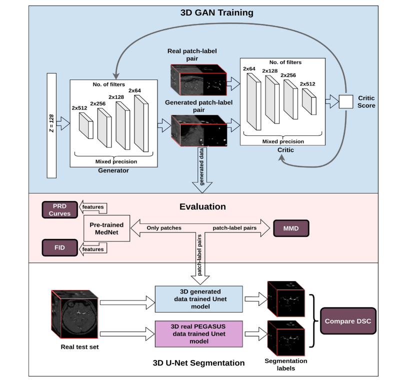
Fig. 1. Structure of the workflow from training the 3D GAN to qualitative and quantitative assessments. Top: Overview of GAN training - Here, we illustrate our most complex model using spectral normalization and mixed precision (c-SN-MP), middle: Evaluation schemes, bottom: Segmentation performance evaluation

圖 1. 從訓練 3D GAN 到定性和定量評估的工作流程結構。頂部：GAN 訓練概覽 - 在此，我們展示了我們使用頻譜歸一化和混合精度的最復雜模型（c-SN-MP），中間：評估方案，底部：分割性能評估。

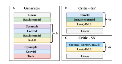
Fig. 2. Architectures of A. Generator of all models, B. Critic of GP model, and C. Critic of all SN models.

圖 2. A. 所有模型的生成器架構，B. GP 模型的批判者架構，以及 C. 所有 SN 模型的批判者架構。

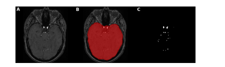
Fig. 3. Brain mask application for intracranial vessels analysis. Here, an axial slice is shown of A. TOF-MRA image with skull B. brain mask extracted using FSL-BET tool from TOF-MRA image C. ground truth segmentation label after brain mask application leading to skull-stripping i.e. removal of all vessels of face and neck with only intracranial vessels remaining

圖 3. 用于顱內血管分析的腦部遮罩應用。這里展示了 A. 帶有頭骨的 TOF-MRA 圖像的軸向切片 B. 使用 FSL-BET 工具從 TOF-MRA 圖像中提取的腦部遮罩 C. 應用腦部遮罩后的地面真實分割標簽，導致去除頭骨，即移除面部和頸部的所有血管，只剩下顱內血管。

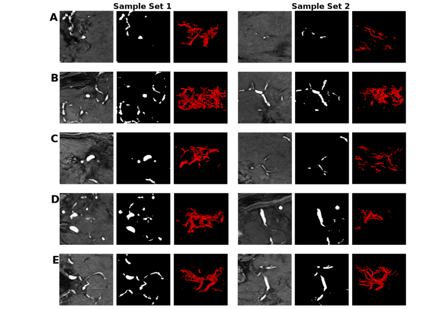
Fig. 4. Sets of samples of the mid-axial slice of the patch and label, and the corresponding 3D vessel structure from A) GP B) SN C) SN-MP D) c-SN-MP and E) real. The visualizations were obtained using ITK-SNAP for illustrative purposes only

圖 4. 來自 A) GP B) SN C) SN-MP D) c-SN-MP 和 E) 真實數據的中軸切片塊和標簽的樣本集合，以及相應的 3D 血管結構。這些可視化是使用 ITK-SNAP 僅出于說明目的而獲得的。

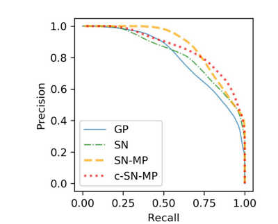
Fig. 5. PRD Curves of synthetic data from the four different models with real data as reference. Precision and Recall in GANs quantify the quality and modes captured by the models respectively

圖 5. 四種不同模型合成數據的 PRD 曲線，以真實數據作為參考。GANs 中的精確度和召回率分別量化了模型捕獲的質量和模式。

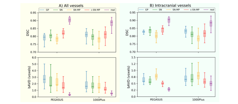
Fig. 6. Segmentation performance (DSC and bAVD) of 3D U-Net models trained with 4 different generated data and PEGASUS training data on the 2 datasets PEGASUS and 1000Plus of A) all vessels B) intracranial vessels. The horizontal line of the box-whisker plots indicates the median, the box indicates the interquartile range and the whiskers the minimum and maximum.

圖6使用 4 種不同生成數據和 PEGASUS 訓練數據在 PEGASUS 和 1000Plus 兩個數據集上訓練的 3D U-Net 模型的分割性能（DSC 和 bAVD），涵蓋 A) 全部血管 B) 顱內血管。箱形圖的水平線表示中位數，箱體表示四分位數范圍，而須表示最小值和最大值。

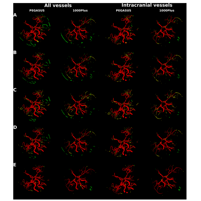
Fig. 7. Segmentation error map of an example patient each from PEGASUS test set and 1000Plus test set for all vessels and for intracranial vessels. Top to bottom maps from 3D U-Net model trained on: A. GP synthetic data B. SN synthetic data C. SN-MP synthetic data D. c-SN-MP synthetic data E. real data. True positives are shown in red, false positives are in green and false negatives in yellow.

圖 7. PEGASUS 測試集和 1000Plus 測試集中每個患者的一個例子的所有血管和顱內血管的分割錯誤圖。從上到下的地圖來自于在以下數據上訓練的 3D U-Net 模型：A. GP 合成數據 B. SN 合成數據 C. SN-MP 合成數據 D. c-SN-MP 合成數據 E. 真實數據。正確的陽性顯示為紅色，錯誤的陽性為綠色，錯誤的陰性為黃色。

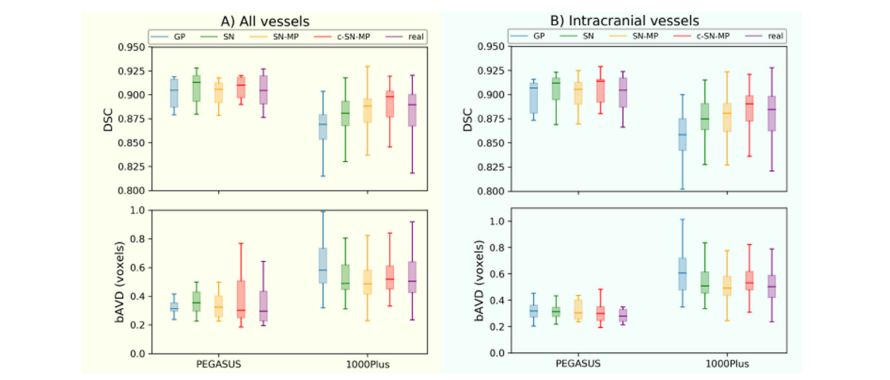
Fig. A.1. Segmentation performance (DSC and bAVD) of 3D U-Net models trained with PEGASUS training data together with 4 different generated data as data augmentation on the 2 datasets PEGASUS and 1000Plus of A) all vessels B) intracranial vessels. The horizontal line of the box-whisker plots indicates the median, the box indicates the interquartile range and the whiskers the minimum and maximum.

圖 A.1. 使用 PEGASUS 訓練數據與 4 種不同生成數據作為數據增強，在 PEGASUS 和 1000Plus 兩個數據集上訓練的 3D U-Net 模型的分割性能（DSC 和 bAVD），涵蓋 A) 全部血管 B) 顱內血管。箱形圖的水平線表示中位數，箱體表示四分位數范圍，而須表示最小值和最大值。

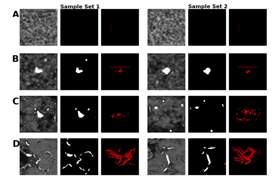
Fig. B.1. Sets of samples of the mid-axial slice of the patch and label, and the corresponding 3D vessel structure from A) DPGAN ≈ 102 B) DPGAN ≈ 103 C) DPGAN ≈ 106 D) real. Note that lower the higher the privacy. The visualizations were obtained using ITK-SNAP for illustrative purposes only.

圖 B.1. 中軸切片的塊和標簽樣本集合，以及來自 A) DPGAN ≈ 102 B) DPGAN ≈ 103 C) DPGAN ≈ 106 D) 真實數據的相應 3D 血管結構。請注意，數值越低，隱私保護程度越高。這些可視化僅使用 ITK-SNAP 出于說明目的而獲得。

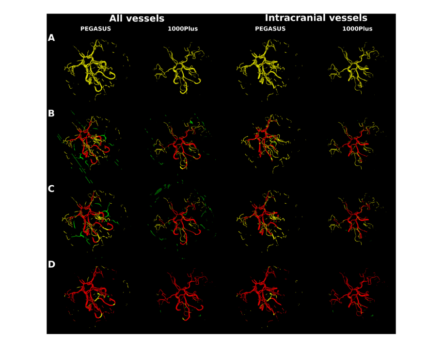
Fig. B.2. Segmentation error map of an example patient each from PEGASUS test set and 1000Plus test set for all vessels and for intracranial vessels. Top to bottom maps from 3D U-Net model trained on: A. DPGAN ≈ 102 B. DPGAN ≈ 103 C. DPGAN ≈ 106 D. real data. True positives are shown in red, false positives are in green and false negatives in yellow、

圖 B.2. PEGASUS 測試集和 1000Plus 測試集中每個患者的一個例子的所有血管和顱內血管的分割錯誤圖。從上到下的地圖來自于在以下數據上訓練的 3D U-Net 模型：A. DPGAN ≈ 102 B. DPGAN ≈ 103 C. DPGAN ≈ 106 D. 真實數據。正確的陽性顯示為紅色，錯誤的陽性為綠色，錯誤的陰性為黃色。

Table

表

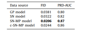
Table 1 FID scores and AUC of the PRD curves for synthetic data from different models.

表 1 不同模型合成數據的 FID 分數和 PRD 曲線的 AUC。

Table 2 Total number of trainable parameters, memory consumption and training times of various 3D GAN models. Note that c-SN-MP, which is our complex mixed precision model, uses twice the number of filters per layer leading to doubling of the trainable parameters compared to non-complex models. The memory consumption increased by 1.5 times compared to the SN model allowing it to be accommodated in the limited memory of our computational infrastructure. The training time also increased by 2.5 times but it was not a constraint in our study

表 2 各種 3D GAN 模型的可訓練參數總數、內存消耗和訓練時間。請注意，我們的復雜混合精度模型 c-SN-MP 每層使用了兩倍數量的濾波器，與非復雜模型相比，可訓練參數數量增加了一倍。與 SN 模型相比，內存消耗增加了 1.5 倍，使其能夠適應我們計算基礎設施的有限內存。訓練時間也增加了 2.5 倍，但在我們的研究中這不是一個限制。

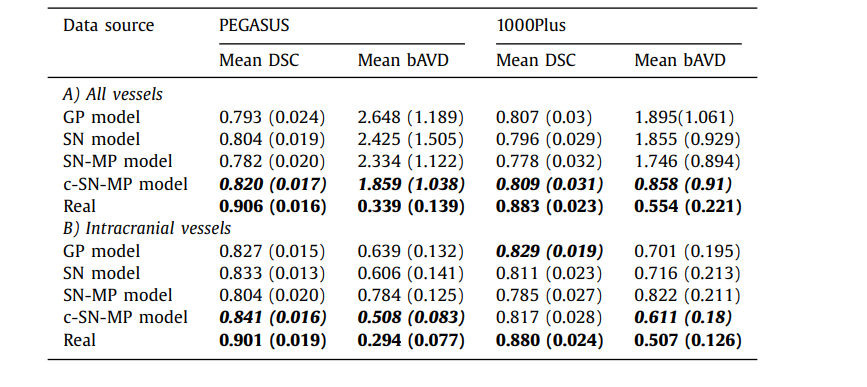
Table 3 The mean DSC and mean bAVD (in voxels) across all the patients in the test set for 2 different datasets PEGASUS and 1000Plus. The value in brackets is the standard deviation across patients. A) All vessels is done on the entire prediction with the entire ground truth as reference, and B) Intracranial vessels is done on skull-stripped prediction with skullstripped ground truth as reference.

表 3 在測試集中所有患者的平均 DSC 和平均 bAVD（以體素計）針對兩個不同的數據集 PEGASUS 和 1000Plus。括號中的值是患者間的標準偏差。A) 全部血管是基于整個預測與整個地面真實作為參考進行的，而 B) 顱內血管是基于去除頭骨的預測與去除頭骨的地面真實作為參考進行的。

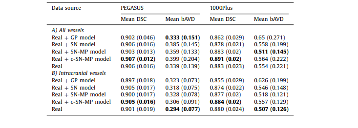
Table A.1 The mean DSC and mean bAVD (in voxels) across all the patients in the test set for 2 different datasets PEGASUS and 1000Plus using model trained with real data along with generated data used as data augmentation. The value in brackets is the standard deviation across patients. A) All vessels is done on the entire prediction with the entire ground truth as reference, and B) Intracranial vessels is done on skull-stripped prediction with skull-stripped ground truth as reference

表 A.1 在測試集中所有患者的平均 DSC 和平均 bAVD（以體素計）針對兩個不同的數據集 PEGASUS 和 1000Plus，使用與真實數據一起訓練的模型，同時生成的數據用作數據增強。括號中的值是患者間的標準偏差。A) 全部血管是基于整個預測與整個地面真實作為參考進行的，而 B) 顱內血管是基于去除頭骨的預測與去除頭骨的地面真實作為參考進行的。

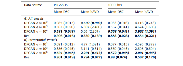
Table B.1 The mean DSC and mean bAVD (in voxels) across all the patients in the test set for 2 different datasets PEGASUS and 1000Plus using model trained with generated data from 3D DPGAN with different values - starting from low value indicating high privacy to the high value indicating low privacy. The value in brackets is the standard deviation across patients. A) All vessels is done on the entire prediction with the entire ground truth as reference, and B) Intracranial vessels is done on skull-stripped prediction with skull-stripped ground truth as reference

All vessels is done on the entire prediction with the entire ground truth as reference, and B) Intracranial vessels is done on skull-stripped prediction with skull-stripped ground truth as reference*

表 B.1 在測試集中所有患者的平均 DSC 和平均 bAVD（以體素計）針對兩個不同的數據集 PEGASUS 和 1000Plus，使用從具有不同 值的 3D DPGAN 生成的數據訓練的模型，從表示高隱私的低 值到表示低隱私的高 值。括號中的值是患者間的標準偏差。A) 全部血管是基于整個預測與整個地面真實作為參考進行的，而 B) 顱內血管是基于去除頭骨的預測與去除頭骨的地面真實作為參考進行的。