Clustering algorithms are a powerful technique for machine learning on unsupervised data. The most common algorithms in machine learning are hierarchical clustering and K-Means clustering. These two algorithms are incredibly powerful when applied to different machine learning problems.

聚類算法是用于在無監督數據上進行機器學習的強大技術。 機器學習中最常見的算法是層次聚類和K-Means聚類。 當將這兩種算法應用于不同的機器學習問題時，它們的功能異常強大。

Cluster analysis can be a powerful data-mining tool for any organization that needs to identify discrete groups of customers, sales transactions, or other types of behaviors and things. For example, insurance providers use cluster analysis to detect fraudulent claims, and banks use it for credit scoring.

對于需要識別離散的客戶組，銷售交易或其他類型的行為和事物的組織， 群集分析可以是功能強大的數據挖掘工具。 例如，保險提供商使用聚類分析來檢測欺詐性索賠，銀行將其用于信用評分。

Algorithm mostly in →

算法主要在→

1. Identification of fake news .
   鑒定假新聞。
2. Spam filter
   垃圾郵件過濾器
3. marketing sales
   市場銷售
4. Classify network traffic.
   分類網絡流量。
5. Identifying fraudulent or criminal activity
   識別欺詐或犯罪活動

Here are the topics we will be covering in this clustering techniques.

這是我們將在此聚類技術中涵蓋的主題。

* PCA Decomposition (Dimensionality Reduction)* K-Means Clustering (Centroid Based) Clustering* Hierarchical (Divisive and Agglomerative) Clustering* DBSCAN (Density Based) Clustering

* PCA分解(降維)* K均值聚類(基于中心)聚類*分層(除法和聚集)聚類* DBSCAN(基于密度)聚類

# Importing Data

＃導入數據

import pandas as pddata = pd.read_csv(‘../input/unsupervised-learning-on-country-data/Country-data.csv’)

將pandas導入為pddata = pd.read_csv('../ input / unsupervised-learning-on-country-data / Country-data.csv')

Let’s check the contents of data

讓我們檢查數據的內容

data.head()

data.head()

#describtion of dataset

＃描述數據集

data.describe()

data.describe()

What do the column headings mean? Let’s check the data dictionary.

列標題是什么意思？ 讓我們檢查數據字典。

import pandas as pddata_dict = pd.read_csv(‘../input/unsupervised-learning-on-country-data/data-dictionary.csv’)data_dict.head(10)

將熊貓作為pddata_dict = pd.read_csv('../ input / unsupervised-learning-on-country-data / data-dictionary.csv')data_dict.head(10)導入

# Analyzing Data

＃分析數據

#Data analysis baseline library!pip install dabl

＃數據分析基準庫！pip install dabl

We are using Data Analysis Baseline Library here. It will help us analyze the data with respect to the target column.

我們在這里使用數據分析基準庫。 這將幫助我們分析有關目標列的數據。

import dablimport warningsimport matplotlib.pyplot as pltwarnings.filterwarnings(‘ignore’)plt.style.use(‘ggplot’)plt.rcParams[‘figure.figsize’] = (12, 6)dabl.plot(data, target_col = ‘gdpp’)

import dablimport warnings將matplotlib.pyplot導入為pltwarnings.filterwarnings('ignore')plt.style.use('ggplot')plt.rcParams ['figure.figsize'] =(12，6)dabl.plot(data，target_col =' gdpp')

We can observe very close positive correlation between “Income” and “GDPP”. Also, “Exports”, “Imports”, “Health” have sort of positive correlation with “GDPP”.

我們可以觀察到“收入”與“ GDPP”之間非常緊密的正相關。 此外，“出口”，“進口”，“健康”與“ GDPP”具有正相關。

However, we will now drop the column “Country” not because it is the only categorical (object type) parameter, but because it is not a deciding parameter to keep/not-keep a particular record within a cluster. In short, “Country” is a feature which is not required here for unsupervised learning.

但是，我們現在將刪除“國家/地區”列，不是因為它是唯一的分類(對象類型)參數，而是因為它不是保留/不保留集群中特定記錄的決定性參數。 簡而言之，“國家/地區”是一種無監督學習所不需要的功能。

# Exclude “Country” columndata = data.drop(‘country’, axis=1)

＃排除“國家”列數據= data.drop('國家'，軸= 1)

We will use simple profile reporting where we can get an easy overview of variables, and we can explore interactions (pair-wise scatter plots), correlations (Pearson’s, Spearman’s, Kendall’s, Phik), missing value information — all in one place. The output it produces is a bit long though, and we need to scroll down and toggle different tabs to view all the results, but the time you spend on it is worth it.

我們將使用簡單的配置文件報告，從中可以輕松了解變量，并可以探索相互作用(成對散點圖)，相關性(皮爾遜氏，斯皮爾曼氏，肯德爾氏，菲克)，價值缺失信息-全部集中在一個地方。 盡管它產生的輸出有點長，我們需要向下滾動并切換不同的選項卡以查看所有結果，但是花在它上面的時間是值得的。

Gist of Overview:

概述要點：

• Average death of children under age 5 in every 100 people: 38.27
  每100人中5歲以下兒童的平均死亡人數：38.27
• Average life expectancy: 70.56 (highly negatively skewed distribution)
  平均壽命：70.56(高度負偏斜分布)
• Health has a perfectly symmetric distribution with mean 6.82
  健康狀況具有完美的對稱分布，平均值為6.82
• Average exports of goods and services per capita: 41.11
  人均商品和服務平均出口：41.11
• Average imports of goods and services per capita: 46.89 (which is > avg. exports)
  人均商品和服務平均進口：46.89(平均出口>)
• Average net income per person: 17144.69 (highly positively skewed distribution)
  人均純收入：17144.69(高度正偏分布)
• Average inflation: 7.78 (has a wide spread ranging from min -4.21 till +104)
  平均通貨膨脹率：7.78(價差最低-4.21到+104)
• Average GDP per capita: 12964.15 (highly negatively skewed distribution)
  人均國內生產總值：12964.15(高度負偏斜分布)

Gist of Interactions:

互動要點：

• Child Mortality has a perfect negative correlation with Life Expectancy
  兒童死亡率與預期壽命具有完全負相關
• Total Fertility has somewhat positive correlation with Child Mortality
  總生育率與兒童死亡率有些正相關
• Exports and Imports have rough positive correlation
  進出口大致呈正相關
• Income and GDPP have fairly positive correlation
  收入與GDPP呈正相關

Gist of Missing Values:

價值缺失要點：

• There is no missing value in data
  數據中沒有缺失值

We will discuss correlation coefficients in detail later.

稍后我們將詳細討論相關系數。

#More prominent correlation plotimport numpy as npimport seaborn as snscorr = data.corr()mask = np.triu(np.ones_like(corr, dtype=np.bool))f, ax = plt.subplots(figsize=(12, 12))cmap = sns.light_palette(‘black’, as_cmap=True)sns.heatmap(corr, mask=mask, cmap=cmap, vmax=None, center=0,square=True, annot=True, linewidths=.5, cbar_kws={“shrink”: .9})

＃更多重要的相關圖將numpy導入為np導入為snscorr = data.corr()掩碼= np.triu(np.ones_like(corr，dtype = np.bool))f，ax = plt.subplots(figsize =(12，12 ))cmap = sns.light_palette('black'，as_cmap = True)sns.heatmap(corr，mask = mask，cmap = cmap，vmax = None，center = 0，square = True，annot = True，線寬= .5 ，cbar_kws = {“收縮”：.9})

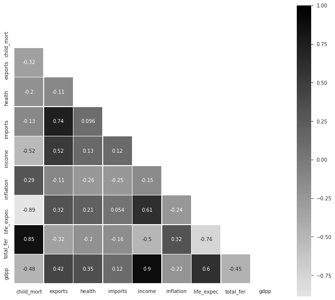
Insights from Pearson’s Correlation Coefficient Plot :

皮爾遜相關系數圖的見解：

• Imports have high positive correlation with Exports (+0.74)
  進口與出口呈高度正相關(+0.74)
• Income has fairly high positive correlation with Exports (+0.52)
  收入與出口呈正相關(+0.52)
• Life Expectancy has fairly high positive correlation with Income (+0.61)
  預期壽命與收入的正相關性很高(+0.61)
• Total Fertility has very high positive correlation with Child Mortality (+0.85)
  總生育率與兒童死亡率有非常高的正相關性(+0.85)
• GDPP has very high positive correlation with Income (+0.90)
  GDPP與收入的正相關性非常高(+0.90)
• GDPP has fairly high positive correlation with Life Expectancy (+0.60)
  GDPP與預期壽命有較高的正相關(+0.60)

• Total Fertility has fairly high negative correlation with Life Expectancy (-0.76) — Well, I found this particular thing as an interesting insight but let’s not forget “Correlation does not imply causation”!

  總生育率與預期壽命(-0.76)具有相當高的負相關性-嗯，我發現這件事很有趣，但請不要忘記“相關性并不意味著因果關系”！

(1)主成分分析 ((1) Principal Component Analysis)

Principal Component Analysis (PCA) is a popular technique for deriving a set of low dimensional features from a large set of variables. Sometimes reduced dimensional set of features can represent distinct no. of groups with similar characteristics. Hence PCA can be an insightful clustering tool (or a preprocessing tool before applying clustering as well). We will standardize our data first and will use the scaled data for all clustering works in future.

主成分分析(PCA)是一種流行的技術，可以從大量變量中得出一組低維特征。 有時，特征的縮小維集可以表示不同的編號。 具有相似特征的群體。 因此，PCA可以是有見地的聚類工具(或在應用聚類之前也可以作為預處理工具)。 我們將首先對數據進行標準化，并在將來將縮放后的數據用于所有聚類工作。

from sklearn.preprocessing import StandardScalersc=StandardScaler()data_scaled=sc.fit_transform(data)

從sklearn.preprocessing導入StandardScalersc = StandardScaler()data_scaled = sc.fit_transform(data)

Here, I have used singular value decomposition solver “auto” to get the no. of principal components. You can also use solver “randomized” introducing a random state seed like “0” or “12345”.

在這里，我使用奇異值分解求解器“ auto”來獲得否。 主要組成部分。 您還可以使用“隨機化”的求解器，引入諸如“ 0”或“ 12345”之類的隨機狀態種子。

from sklearn.decomposition import PCApc = PCA(svd_solver=’auto’)pc.fit(data_scaled)print(‘Total no. of principal components =’,pc.n_components_)

從sklearn.decomposition導入PCApc = PCA(svd_solver ='auto')pc.fit(data_scaled)print('主組件總數='，pc.n_components_)

#Print Principal Componentsprint(‘Principal Component Matrix :\n’,pc.components_)

#Print主要組件print('主要組件矩陣：\ n'，pc.components_)

Let us check the amount of variance explained by each principal component here. They will be arranged in decreasing order of their explained variance ratio.

讓我們在這里檢查每個主成分所解釋的方差量。 它們將按其解釋的方差比的降序排列。

#The amount of variance that each PC explainsvar = pc.explained_variance_ratio_print(var)

＃每臺PC解釋的方差量var = pc.explained_variance_ratio_print(var)

#Plot explained variance ratio for each PCplt.bar([i for i, _ in enumerate(var)],var,color=’black’)plt.title(‘PCs and their Explained Variance Ratio’, fontsize=15)plt.xlabel(‘Number of components’,fontsize=12)plt.ylabel(‘Explained Variance Ratio’,fontsize=12)

＃繪制每個PC的解釋方差比率plt.bar([i代表i，_枚舉(var)]，var，color ='black')plt.title('PC及其解釋方差比率'，fontsize = 15) plt.xlabel('組件數'，fontsize = 12)plt.ylabel('Explained Variance Ratio'，fontsize = 12)

Using these cumulative variance ratios for all PCs, we will now draw a scree plot. It is used to determine the number of principal components to keep in this principal component analysis.

使用所有PC的這些累積方差比，我們現在將繪制一個scree圖。 用于確定要保留在此主成分分析中的主成分數。

# Scree Plotplt.plot(cum_var, marker=’o’)plt.title(‘Scree Plot: PCs and their Cumulative Explained Variance Ratio’,fontsize=15)plt.xlabel(‘Number of components’,fontsize=12)plt.ylabel(‘Cumulative Explained Variance Ratio’,fontsize=12)

＃Scree Plotplt.plot(cum_var，marker ='o')plt.title('Scree Plot：PC及其累積解釋方差比'，fontsize = 15)plt.xlabel('components'，fontsize = 12)plt .ylabel('累積解釋方差比'，fontsize = 12)

The plot indicates the threshold of 90% is getting crossed at PC = 4. Ideally, we can keep 4 (or atmost 5) components here. Before PC = 5, the plot is following an upward trend. After crossing 5, it is almost steady. However, we have retailed all 9 PCs here to get the full data in results. And for visualization purpose in 2-D figure, we have plotted only PC1 vs PC2.

該圖表明在PC = 4時超過了90％的閾值。理想情況下，此處可以保留4個(或最多5個)組件。 在PC = 5之前，該圖遵循上升趨勢。 越過5后，它幾乎保持穩定。 但是，我們在這里零售了所有9臺PC，以獲取完整的數據結果。 并且出于二維圖的可視化目的，我們僅繪制了PC1 vs PC2。

#Principal Component Data Decompositioncolnames = list(data.columns)pca_data = pd.DataFrame({ ‘Features’:colnames,’PC1':pc.components_[0],’PC2':pc.components_[1],’PC3':pc.components_[2], ‘PC4’:pc.components_[3],’PC5':pc.components_[4], ‘PC6’:pc.components_[5], ‘PC7’:pc.components_[6], ‘PC8’:pc.components_[7], ‘PC9’:pc.components_[8]})pca_data

＃主組件數據分解colnames = list(data.columns)pca_data = pd.DataFrame({'Features'：colnames，'PC1'：pc.components_ [0]，'PC2'：pc.components_ [1]，'PC3' ：pc.components_ [2]，'PC4'：pc.components_ [3]，'PC5'：pc.components_ [4]，'PC6'：pc.components_ [5]，'PC7'：pc.components_ [6 ]，“ PC8”：pc.components_ [7]，“ PC9”：pc.components_ [8]})pca_data

we will se then

然后我們會

#Visualize 2 main PCsfig = plt.figure(figsize = (12,6))sns.scatterplot(pca_data.PC1, pca_data.PC2,hue=pca_data.Features,marker=’o’, s=500)plt.title(‘PC1 vs PC2’,fontsize=15)plt.xlabel(‘Principal Component 1’,fontsize=12)plt.ylabel(‘Principal Component 2’,fontsize=12)plt.show()

＃可視化2個主要PCsfig = plt.figure(figsize =(12,6))sns.scatterplot(pca_data.PC1，pca_data.PC2，hue = pca_data.Features，marker ='o'，s = 500)plt.title( 'PC1 vs PC2'，fontsize = 15)plt.xlabel('主組件1'，fontsize = 12)plt.ylabel('主組件2'，fontsize = 12)plt.show()

We can see that 1st Principal Component (X-axis) is gravitated mainly towards features like: life expectancy, gdpp, income. 2nd Principal Component (Y-axis) is gravitated predominantly towards features like: imports, exports.

我們可以看到，第一主成分(X軸)主要受以下特征的影響：預期壽命，gdpp和收入。 第二主要組成部分(Y軸)主要具有以下特征：導入，導出。

#Export PCA results to filepca_data.to_csv(“PCA_results.csv”, index=False)

＃將PCA結果導出到filepca_data.to_csv(“ PCA_results.csv”，index = False)

(2) K-Means Clustering

(2)K-均值聚類

This is the most popular method of clustering. It uses Euclidean distance between clusters in each iteration to decide a data point should belong to which cluster, and proceed accordingly. To decide how many no. of clusters to consider, we can employ several methods. The basic and most widely used method is **Elbow Curve**.

這是最流行的群集方法。 它在每次迭代中使用簇之間的歐式距離來確定數據點應屬于哪個簇，然后進行相應處理。 決定多少不。 考慮集群，我們可以采用幾種方法。 基本且使用最廣泛的方法是“肘曲線”。

**Method-1: Plotting Elbow Curve**

**方法1：繪制肘曲線**

In this curve, wherever we observe a “knee” like bent, we can take that number as the ideal no. of clusters to consider in K-Means algorithm.

在此曲線中，無論何時我們觀察到像彎曲一樣的“膝蓋”，我們都可以將該數字作為理想編號。 K-Means算法中要考慮的群集數量。

from yellowbrick.cluster import KElbowVisualizer

從yellowbrick.cluster導入KElbowVisualizer

#Plotting Elbow Curvefrom sklearn.cluster import KMeansfrom yellowbrick.cluster import KElbowVisualizerfrom sklearn import metrics

＃從sklearn.cluster導入彎頭曲線從yellowbrick.cluster導入KMeans從sklearn導入指標導入KElbowVisualizer

model = KMeans()visualizer = KElbowVisualizer(model, k=(1,10))visualizer.fit(data_scaled) visualizer.show()

模型= KMeans()可視化器= KElbowVisualizer(模型，k =(1,10))可視化器.fit(數據縮放)可視化器.show()

Here, along Y-axis, “distortion” is defined as “the sum of the squared differences between the observations and the corresponding centroid”. It is same as WCSS (Within-Cluster-Sum-of-Squares).

在此，沿Y軸的“變形”被定義為“觀測值與對應的質心之間的平方差的和”。 它與WCSS(集群內平方和)相同。

Let’s see the centroids of the clusters. Afterwards, we will fit our scaled data into a K-Means model having 3 clusters, and then label each data point (each record) to one of these 3 clusters.

讓我們看一下群集的質心。 然后，我們將縮放后的數據擬合到具有3個聚類的K-Means模型中，然后將每個數據點(每個記錄)標記為這3個聚類之一。

#Fitting data into K-Means model with 3 clusterskm_3=KMeans(n_clusters=3,random_state=12345)km_3.fit(data_scaled)print(km_3.cluster_centers_)

＃將數據擬合到具有3個簇的K-Means模型中km_3 = KMeans(n_clusters = 3，random_state = 12345)km_3.fit(data_scaled)print(km_3.cluster_centers_)

We can see each record has got a label among 0,1,2. This label is each of their cluster_id i.e. in which cluster they belong to. We can count the records in each cluster now.

我們可以看到每個記錄在0,1,2之間都有一個標簽。 該標簽是它們的每個cluster_id，即它們所屬的集群。 我們現在可以計算每個群集中的記錄。

pd.Series(km_3.labels_).value_counts()

pd.Series(km_3.labels _)。value_counts()

We see, the highest no. of records belong to the first cluster.

我們看到，最高的沒有。 的記錄屬于第一個群集。

Now, we are interested to check how good is our K-Means clustering model. Silhouette Coefficient is one such metric to check that. The **Silhouette Coefficient** is calculated using: * the mean intra-cluster distance ( a ) for each sample* the mean nearest-cluster distance ( b ) for each sample* The Silhouette Coefficient for a sample is (b — a) / max(a, b)

現在，我們有興趣檢查我們的K-Means聚類模型的性能如何。 輪廓系數就是一種用于檢驗這一指標的指標。 **剪影系數**使用以下公式計算：*每個樣本的平均集群內距離(a)*每個樣本的平均最近集群距離(b)*樣本的剪影系數為(b — a) /最大(a，b)

# calculate Silhouette Coefficient for K=3from sklearn import metricsmetrics.silhouette_score(data_scaled, km_3.labels_)

＃從sklearn導入指標metrics.silhouette_score(data_scaled，km_3.labels_)計算K = 3的輪廓系數

# calculate SC for K=2 through K=10k_range = range(2, 10)scores = []for k in k_range: km = KMeans(n_clusters=k, random_state=12345) km.fit(data_scaled) scores.append(metrics.silhouette_score(data_scaled, km.labels_))

＃計算K = 2到K = 10的SC k_range = range(2，10)分數= [] k中k的k：km = KMeans(n_clusters = k，random_state = 12345)km.fit(data_scaled)scores.append(metrics) .silhouette_score(data_scaled，km.labels_))

We observe the highest silhouette score with no. of clusters 3 and 4. However, from Elbow Curve, we got to see the “knee” like bent at no. of clusters 3. So we will do further analysis to choose the ideal no. of clusters between 3 and 4.

我們觀察到最高的輪廓得分，沒有。 圖3和4中的曲線。但是，從肘彎曲線，我們可以看到“膝蓋”像彎腰一樣彎曲。 因此，我們將做進一步分析以選擇理想編號。 在3到4之間的集群。

For further analysis, we will consider **Davies-Bouldin Score** apart from Silhouette Score. **Davies-Bouldin Score** is defined as the average similarity measure of each cluster with its most similar cluster, where similarity is the ratio of within-cluster distances to between-cluster distances. Thus, clusters which are farther apart and less dispersed will result in a better score.

為了進一步分析，我們將考慮“ Davies-Bouldin得分” **(除了“剪影得分”)。 戴維斯-布爾丁得分**定義為每個群集與其最相似群集的平均相似性度量，其中相似度是群集內距離與群集間距離之比。 因此，距離較遠且分散程度較低的群集將獲得更好的分數。

We will also analyze **SSE (Sum of Squared Errors)**. SSE is the sum of the squared differences between each observation and its cluster’s mean. It can be used as a measure of variation within a cluster. If all cases within a cluster are identical the SSE would then be equal to 0. The formula for SSE is: 1

我們還將分析** SSE(平方誤差總和)**。 SSE是每個觀察值與其簇的均值之間平方差的總和。 它可以用作衡量群集內變化的指標。 如果集群中的所有情況都相同，則SSE等于0。SSE的公式為：1

Method-2: Plotting of SSE, Davies-Bouldin Scores, Silhouette Scores to Decide Ideal No. of Clusters

方法2：繪制SSE，Davies-Bouldin分數，Silhouette分數以確定理想的聚類數

from sklearn.metrics import davies_bouldin_score, silhouette_score, silhouette_samplessse,db,slc = {}, {}, {}for k in range(2, 10): kmeans = KMeans(n_clusters=k, max_iter=1000,random_state=12345).fit(data_scaled) if k == 4: labels = kmeans.labels_ clusters = kmeans.labels_ sse[k] = kmeans.inertia_ # Inertia: Sum of distances of samples to their closest cluster center db[k] = davies_bouldin_score(data_scaled,clusters) slc[k] = silhouette_score(data_scaled,clusters)

從sklearn.metrics導入davies_bouldin_score，silhouette_score，silhouette_samplessse，db，slc = {}，{}，{}對于范圍(2，10)中的k：kmeans = KMeans(n_clusters = k，max_iter = 1000，random_state = 12345)。如果k == 4，則擬合(data_scaled)：標簽= kmeans.labels_群集= kmeans.labels_ sse [k] = kmeans.inertia_＃慣性：樣本到其最近的群集中心的距離之和db [k] = davies_bouldin_score(data_scaled，群集)slc [k] = silhouette_score(data_scaled，clusters)

#Plotting SSEplt.figure(figsize=(12,6))plt.plot(list(sse.keys()), list(sse.values()))plt.xlabel(“Number of cluster”, fontsize=12)plt.ylabel(“SSE (Sum of Squared Errors)”, fontsize=12)plt.title(“Sum of Squared Errors vs No. of Clusters”, fontsize=15)plt.show()

＃繪制SSEplt.figure(figsize =(12,6))plt.plot(list(sse.keys())，list(sse.values()))plt.xlabel(“簇數”，fontsize = 12) plt.ylabel(“ SSE(平方誤差之和)”，fontsize = 12)plt.title(“平方誤差之和與簇數”，fontsize = 15)plt.show()

We can see “knee” like bent at both 3 and 4, still considering no. of clusters = 4 seems a better choice, because after 4, there is no further “knee” like bent observed. Still, we will analyse further to decide between 3 and 4.

我們可以看到“膝蓋”在第3和第4處都彎曲了，但仍不考慮。 簇= 4似乎是一個更好的選擇，因為在4之后，不再觀察到像彎曲一樣的“膝蓋”。 不過，我們將進一步分析以決定3到4。

#Plotting Davies-Bouldin Scoresplt.figure(figsize=(12,6))plt.plot(list(db.keys()), list(db.values()))plt.xlabel(“Number of cluster”, fontsize=12)plt.ylabel(“Davies-Bouldin values”, fontsize=12)plt.title(“Davies-Bouldin Scores vs No. of Clusters”, fontsize=15)plt.show()

＃繪制Davies-Bouldin Scoresplt.figure(figsize =(12,6))plt.plot(list(db.keys())，list(db.values()))plt.xlabel(“簇數”，字體大小= 12)plt.ylabel(“ Davies-Bouldin值”，fontsize = 12)plt.title(“ Davies-Bouldin分數與簇數”，fontsize = 15)plt.show()

clearly no choice for =3 in best choice.

顯然，最佳選擇中沒有選擇= 3。

plt.figure(figsize=(12,6))plt.plot(list(slc.keys()), list(slc.values()))plt.xlabel(“Number of cluster”, fontsize=12)plt.ylabel(“Silhouette Score”, fontsize=12)plt.title(“Silhouette Score vs No. of Clusters”, fontsize=15)plt.show()

plt.figure(figsize =(12,6))plt.plot(list(slc.keys())，list(slc.values()))plt.xlabel(“簇數”，fontsize = 12)plt。 ylabel(“ Silhouette Score”，fontsize = 12)plt.title(“ Silhouette Score vs. No. of Clusters”，fontsize = 15)plt.show()

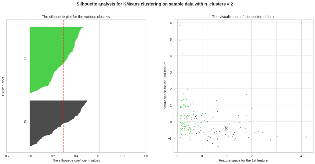
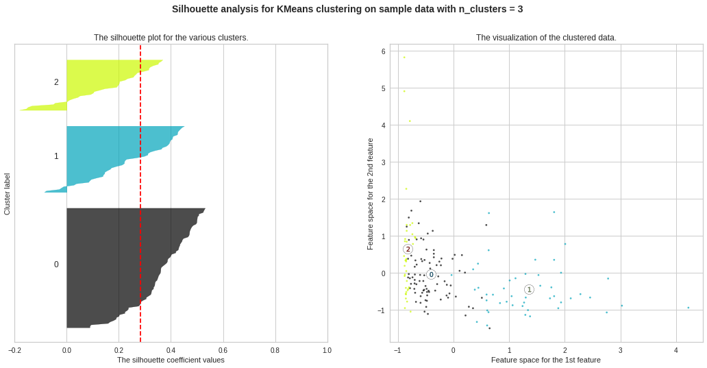
No. of clusters = 3 seems the best choice here as well. The silhouette score ranges from ?1 to +1, where a high value indicates that the object is well matched to its own cluster and poorly matched to neighboring clusters. A score nearly 0.28 seems a good one.

簇數= 3似乎也是這里的最佳選擇。 輪廓分數從-1到+1，其中較高的值表示對象與其自身的群集匹配良好，而與相鄰群集的匹配較差。 接近0.28的分數似乎是一個不錯的成績。

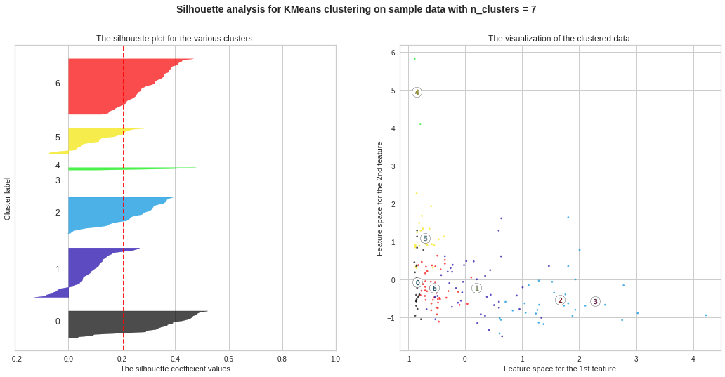
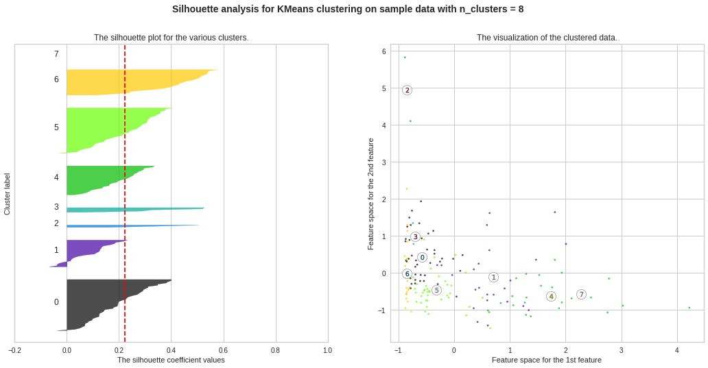
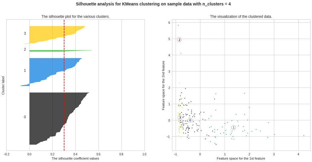
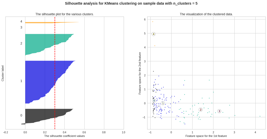
Silhouette Plots for Different No. of Clusters :**We will now draw Silhouette Plots for different no. of clusters for getting more insights. Side by side, we will observe the shape of the clusters in 2-dimensional figure.

不同數量簇的輪廓圖：**我們現在將繪制不同數量簇的輪廓圖。 以獲得更多的見解。 并排，我們將在二維圖中觀察簇的形狀。

#Silhouette Plots for Different No. of Clustersimport matplotlib.cm as cmimport numpy as npfor n_clusters in range(2, 10): fig, (ax1, ax2) = plt.subplots(1, 2) fig.set_size_inches(18, 8) # The 1st subplot is the silhouette plot # The silhouette coefficient can range from -1, 1 but here the range is from -0.2 till 1 ax1.set_xlim([-0.2, 1]) # The (n_clusters+1)*10 is for inserting blank space between silhouette plots of individual clusters, to demarcate them clearly. ax1.set_ylim([0, len(data_scaled) + (n_clusters + 1) * 10]) # Initialize the clusterer with n_clusters value and a random generator seed of 12345 for reproducibility. clusterer = KMeans(n_clusters=n_clusters,max_iter=1000, random_state=12345) cluster_labels = clusterer.fit_predict(data_scaled) # The silhouette_score gives the average value for all the samples # This gives a perspective into the density and separation of the formed clusters silhouette_avg = silhouette_score(data_scaled, cluster_labels) print(“For n_clusters =”, n_clusters, “The average silhouette_score is :”, silhouette_avg) # Compute the silhouette scores for each sample sample_silhouette_values = silhouette_samples(data_scaled, cluster_labels) y_lower = 10 for i in range(n_clusters): # Aggregate the silhouette scores for samples belonging to cluster i and sort them ith_cluster_silhouette_values = sample_silhouette_values[cluster_labels == i] ith_cluster_silhouette_values.sort() size_cluster_i = ith_cluster_silhouette_values.shape[0] y_upper = y_lower + size_cluster_i color = cm.nipy_spectral(float(i) / n_clusters) ax1.fill_betweenx(np.arange(y_lower, y_upper), 0, ith_cluster_silhouette_values, facecolor=color, edgecolor=color, alpha=0.7)

＃不同簇數的剪影圖將matplotlib.cm作為cmimport numpy作為np表示npclus在范圍(2，10)中的n_clusters：fig，(ax1，ax2)= plt.subplots(1，2)圖set_size_inches(18，8) ＃第一個子圖是輪廓圖＃輪廓系數的范圍可以是-1，1，但是這里的范圍是-0.2到1 ax1.set_xlim([-0.2，1])＃(n_clusters + 1)* 10是用于在各個群集的輪廓圖之間插入空白，以清楚地對其進行劃分。 ax1.set_ylim([0，len(data_scaled)+(n_clusters + 1)* 10])＃使用n_clusters值和12345的隨機生成器種子初始化集群器，以實現可重復性。 clusterer = KMeans(n_clusters = n_clusters，max_iter = 1000，random_state = 12345)cluster_labels = clusterer.fit_predict(data_scaled)＃silhouette_score給出了所有樣本的平均值＃這是透視形成的簇的密度和分離度的輪廓silhouette_avg = silhouette_score(data_scaled，cluster_labels)print(“對于n_clusters =”，n_clusters，“平均silhouette_score為：”，silhouette_avg)＃計算每個樣本sample_silhouette_values的輪廓分數= Silhouette_samples(data_scaled，cluster_labels)y_lower = 10代表i (n_clusters)：＃匯總屬于群集i的樣本的輪廓分數，并對其進行排序。 (float(i)/ n_clusters)ax1.fill_betweenx(np.arange(y_lower，y_upper)，0，ith_cluster_silhou ette_values，facecolor = color，edgecolor = color，alpha = 0.7)

# Label the silhouette plots with their cluster numbers at the middle ax1.text(-0.05, y_lower + 0.5 * size_cluster_i, str(i))

＃在輪廓圖的中間ax1.text(-0.05，y_lower + 0.5 * size_cluster_i，str(i))上標記輪廓圖

# Compute the new y_lower for next plot y_lower = y_upper + 10

＃計算下一個圖的新y_lower y_lower = y_upper + 10

ax1.set_title(“The silhouette plot for the various clusters.”) ax1.set_xlabel(“The silhouette coefficient values”) ax1.set_ylabel(“Cluster label”)

ax1.set_title(“各個群集的輪廓圖。”)ax1.set_xlabel(“輪廓系數值”)ax1.set_ylabel(“群集標簽”)

# The vertical line for average silhouette score of all the values ax1.axvline(x=silhouette_avg, color=”red”, linestyle=” — “)

＃所有值ax1.axvline(x = silhouette_avg，color =“ red”，linestyle =” —“)的平均輪廓分數的垂直線

ax1.set_yticks([]) # Clear the yaxis labels ax1.set_xticks([-0.2, 0, 0.2, 0.4, 0.6, 0.8, 1])

ax1.set_yticks([])＃清除yaxis標簽ax1.set_xticks([-0.2，0，0.2，0.4，0.6，0.8，1])

# 2nd Plot showing the actual clusters formed colors = cm.nipy_spectral(cluster_labels.astype(float) / n_clusters) ax2.scatter(data_scaled[:, 0], data_scaled[:, 1], marker=’.’, s=30, lw=0, alpha=0.7, c=colors, edgecolor=’k’)

＃2nd圖顯示了實際的群集形成的顏色= cm.nipy_spectral(cluster_labels.astype(float)/ n_clusters)ax2.scatter(data_scaled [:, 0]，data_scaled [:, 1]，marker ='。'，s = 30 ，lw = 0，alpha = 0.7，c =顏色，edgecolor ='k')

# Labeling the clusters centers = clusterer.cluster_centers_ # Draw white circles at cluster centers ax2.scatter(centers[:, 0], centers[:, 1], marker=’o’, c=”white”, alpha=1, s=200, edgecolor=’k’)

＃標記聚類中心= clusterer.cluster_centers_＃在聚類中心ax2.scatter(centers [:, 0]，center [:, 1]，marker ='o'，c =“ white”，alpha = 1， s = 200，edgecolor ='k')

for i, c in enumerate(centers): ax2.scatter(c[0], c[1], marker=’$%d$’ % i, alpha=1, s=50, edgecolor=’k’)

對于i，enumerate(centers)中的c：ax2.scatter(c [0]，c [1]，marker ='$％d $'％i，alpha = 1，s = 50，edgecolor ='k')

ax2.set_title(“The visualization of the clustered data.”) ax2.set_xlabel(“Feature space for the 1st feature”) ax2.set_ylabel(“Feature space for the 2nd feature”)

ax2.set_title(“集群數據的可視化。”)ax2.set_xlabel(“第一個特征的特征空間”)ax2.set_ylabel(“第二個特征的特征空間”)

plt.suptitle((“Silhouette analysis for KMeans clustering on sample data with n_clusters = %d” % n_clusters), fontsize=14, fontweight=’bold’)

plt.suptitle((“使用n_clusters =％d”對樣本數據進行KMeans聚類的剪影分析”％n_clusters)，fontsize = 14，fontweight ='bold')

plt.show()

plt.show()

preds = km_3.labels_data_df = pd.DataFrame(data)data_df[‘KM_Clusters’] = predsdata_df.head(10)

preds = km_3.labels_data_df = pd.DataFrame(數據)data_df ['KM_Clusters'] = predsdata_df.head(10)

We will visualize 3 clusters now for various pairs of features. Initially, I chose the pairs randomly. Later, I chose the pairs including “GDPP”, “income”, “inflation” etc. important features. Since we are concerned about analyzing country profiles and “GDPP” is the main indicator to represent a country’s status, we are concerned with that mainly.

現在，我們將可視化3個群集，以顯示各種功能對。 最初，我是隨機選擇的。 后來，我選擇了包括“ GDPP”，“收入”，“通貨膨脹”等重要特征的貨幣對。 由于我們關注分析國家概況，“ GDPP”是代表一個國家地位的主要指標，因此我們主要關注這一點。

#Visualize clusters: Feature Pair-1import matplotlib.pyplot as plt_1plt_1.rcParams[‘axes.facecolor’] = ‘lightblue’plt_1.figure(figsize=(12,6))plt_1.scatter(data_scaled[:,0],data_scaled[:,1],c=cluster_labels) #child mortality vs exportsplt_1.title(“Child Mortality vs Exports (Visualize KMeans Clusters)”, fontsize=15)plt_1.xlabel(“Child Mortality”, fontsize=12)plt_1.ylabel(“Exports”, fontsize=12)plt_1.rcParams[‘axes.facecolor’] = ‘lightblue’plt_1.show()

#Visualize clusters：Feature Pair-1import matplotlib.pyplot as plt_1plt_1.rcParams ['axes.facecolor'] ='lightblue'plt_1.figure(figsize =(12,6))plt_1.scatter(data_scaled [：，0]，data_scaled [：，1]，c = cluster_labels)＃兒童死亡率vs出口plt_1.title(“兒童死亡率vs出口(可視化KMeans簇)”，字體大小= 15)plt_1.xlabel(“兒童死亡率”，fontsize = 12)plt_1.ylabel (“導出”，fontsize = 12)plt_1.rcParams ['axes.facecolor'] ='lightblue'plt_1.show()

層次聚類 (Hierarchical clustering)

There are two types of hierarchical clustering: **Divisive** and **Agglomerative**. In divisive (top-down) clustering method, all observations are assigned to a single cluster and then that cluster is partitioned to two least similar clusters, and then those two clusters are partitioned again to multiple clusters, and thus the process go on. In agglomerative (bottom-up), the opposite approach is followed. Here, the ideal no. of clusters is decided by **dendrogram**.

有兩種類型的層次結構聚類：“分裂”和“聚集”。 在分裂(自上而下)的聚類方法中，所有觀察值都分配給一個聚類，然后將該聚類劃分為兩個最不相似的聚類，然后將這兩個聚類再次劃分為多個聚類，因此過程繼續進行。 在團聚(自下而上)中，采用相反的方法。 在這里，理想沒有。 群集的數量由“樹狀圖”決定。

Method-1: Dendrogram Plotting using Clustermap

方法1：使用Clustermap繪制樹狀圖

import seaborn as snscmap = sns.cubehelix_palette(as_cmap=True, rot=-.3, light=1)g = sns.clustermap(data_scaled, cmap=cmap, linewidths=.5)

將seaborn導入為snscmap = sns.cubehelix_palette(as_cmap = True，rot =-。3，light = 1)g = sns.clustermap(data_scaled，cmap = cmap，線寬= .5)

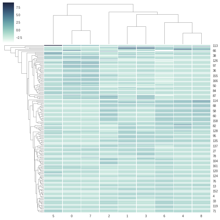
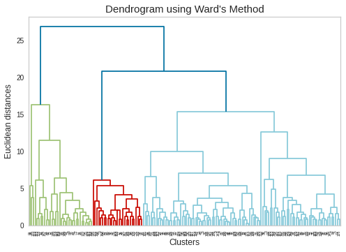
From above dendrogram, we can consider 2 clusters at minimum or 6 clusters at maximum. We will again cross-check the dendrogram using **Ward’s Method**. Ward’s method is an alternative to single-link clustering. This algorithm works for finding a partition with small sum of squares (to minimise the within-cluster-variance).

從上面的樹狀圖中，我們可以考慮最少2個群集或最多6個群集。 我們將再次使用“沃德法”來交叉檢查樹狀圖。 Ward的方法是單鏈接群集的替代方法。 該算法用于查找平方和較小的分區(以最大程度地減少集群內方差)。

Method-2: Dendrogram Plotting using Ward’s Method

方法2：使用Ward方法繪制樹狀圖

# Using the dendrogram to find the optimal number of clustersimport scipy.cluster.hierarchy as sch

＃使用樹狀圖找到最佳集群數，將scipy.cluster.hierarchy導入為sch

plt.rcParams[‘axes.facecolor’] = ‘white’plt.rcParams[‘axes.grid’] = Falsedendrogram = sch.dendrogram(sch.linkage(data_scaled, method=’ward’))plt.title(“Dendrogram using Ward’s Method”, fontsize=15)plt.xlabel(‘Clusters’, fontsize=12)plt.ylabel(‘Euclidean distances’, fontsize=12)plt.rcParams[‘axes.facecolor’] = ‘white’plt.rcParams[‘axes.grid’] = Falseplt.show()

plt.rcParams ['axes.facecolor'] ='white'plt.rcParams ['axes.grid'] = Falsedendrogram = sch.dendrogram(sch.linkage(data_scaled，method ='ward'))plt.title(“樹狀圖使用Ward方法”，fontsize = 15)plt.xlabel(“簇”，fontsize = 12)plt.ylabel(“歐幾里得距離”，fontsize = 12)plt.rcParams ['axes.facecolor'] ='white'plt。 rcParams ['axes.grid'] = Falseplt.show()

DBSCAN集群 (DBSCAN Clustering)

DBSCAN is an abbreviation of “Density-based spatial clustering of applications with noise”. This algorithm groups together points that are close to each other based on a distance measurement (usually Euclidean distance) and a minimum number of points. It also marks noise as outliers (noise means the points which are in low-density regions).

DBSCAN是“基于噪聲的應用程序的基于密度的空間聚類”的縮寫。 該算法基于距離測量(通常是歐幾里得距離)和最少數量的點將彼此靠近的點組合在一起。 它還將噪聲標記為離群值(噪聲表示低密度區域中的點)。

I found an interesting result with DBSCAN when I used all features of country data. It gave me a single cluster.** I presume, that was very evident to happen because our data is almost evenly spread, so density wise, this algorithm could not bifurcate the datapoints into more than one cluster. Hence, I used only the features which have high correlation with “GDPP”. I also kept “Child Mortality” and “Total Fertility” in my working dataset since they have polarizations — some data points have extremely high values, some have extremely low values (ref. to corresponding scatter plots in data profiling section in the beginning).

使用國家/地區數據的所有功能時，使用DBSCAN發現了一個有趣的結果。 它給了我一個集群。**我想，這是很明顯的，因為我們的數據幾乎均勻地散布了，所以從密度的角度來看，該算法不能將數據點分為多個集群。 因此，我只使用了與“ GDPP”具有高度相關性的特征。 我也將“兒童死亡率”和“總生育率”保留在我的工作數據集中，因為它們存在兩極分化-一些數據點具有極高的值，有些數據點具有極低的值(請參閱開頭的數據分析部分中的相應散點圖)。

from sklearn.cluster import DBSCANimport sklearn.utilsfrom sklearn.preprocessing import StandardScaler

從sklearn.cluster導入DBSCAN從sklearn.preprocessing導入sklearn.utils導入StandardScaler

Clus_dataSet = data[[‘child_mort’,’exports’,’health’,’imports’,’income’,’inflation’,’life_expec’,’total_fer’,’gdpp’]]Clus_dataSet = np.nan_to_num(Clus_dataSet)Clus_dataSet = np.array(Clus_dataSet, dtype=np.float64)Clus_dataSet = StandardScaler().fit_transform(Clus_dataSet)

Clus_dataSet = data [['child_mort'，'exports'，'health'，'imports'，'income'，'inflation'，'life_expec'，'total_fer'，'gdpp']] Clus_dataSet = np.nan_to_num(Clus_dataSet) Clus_dataSet = np.array(Clus_dataSet，dtype = np.float64)Clus_dataSet = StandardScaler()。fit_transform(Clus_dataSet)

# Compute DBSCANdb = DBSCAN(eps=1, min_samples=3).fit(Clus_dataSet)core_samples_mask = np.zeros_like(db.labels_)core_samples_mask[db.core_sample_indices_] = Truelabels = db.labels_#data[‘Clus_Db’]=labels

＃計算DBSCANdb = DBSCAN(eps = 1，min_samples = 3).fit(C??lus_dataSet)core_samples_mask = np.zeros_like(db.labels_)core_samples_mask [db.core_sample_indices_] = Truelabels = db.labels_＃data ['Clus_Db'] =標簽

realClusterNum=len(set(labels)) — (1 if -1 in labels else 0)clusterNum = len(set(labels))

realClusterNum = len(set(labels))—(如果標簽中為-1，則為1，否則為0)clusterNum = len(set(labels))

# A sample of clustersprint(data[[‘child_mort’,’exports’,’health’,’imports’,’income’,’inflation’,’life_expec’,’total_fer’,’gdpp’]].head())

＃clustersprint(data [['child_mort'，'exports'，'health'，'imports'，'income'，'inflation'，'life_expec'，'total_fer'，'gdpp']]。head()的樣本)

# number of labelsprint(“number of labels: “, set(labels))

＃標簽數量print(“標簽數量：”，set(標簽))

We have got 7 clusters using density based clustering which is a distinct observation (7 is much higher than 3 which we got in all three different clustering algorithms we used earlier).

我們使用基于密度的聚類得到了7個聚類，這是一個明顯的觀察結果(其中7個遠遠高于我們之前使用的所有三種不同聚類算法中的3個)。

# save the cluster labels and sort by clusterdatacopy = data.copy()datacopy = datacopy.drop(‘KM_Clusters’, axis=1)datacopy[‘DB_cluster’] = db.labels_

＃保存集群標簽并按clusterdata進行排序datacopy = data.copy()datacopy = datacopy.drop('KM_Clusters'，axis = 1)datacopy ['DB_cluster'] = db.labels_

#Visualize clusters: Random Feature Pair-1 (income vs gdpp)import matplotlib.pyplot as plt_3plt_3.rcParams[‘axes.facecolor’] = ‘orange’plt_3.figure(figsize=(12,6))plt_3.scatter(datacopy[‘income’],datacopy[‘gdpp’],c=db.labels_) plt_3.title(‘Income vs GDPP (Visualize DBSCAN Clusters)’, fontsize=15)plt_3.xlabel(“Income”, fontsize=12)plt_3.ylabel(“GDPP”, fontsize=12)plt_3.rcParams[‘axes.facecolor’] = ‘orange’plt_3.show()

＃可視化群集：隨機特征對1(收入vs gdpp)導入matplotlib.pyplot作為plt_3plt_3.rcParams ['axes.facecolor'] ='orange'plt_3.figure(figsize =(12,6))plt_3.scatter(datacopy ['income']，datacopy ['gdpp']，c = db.labels_)plt_3.title('Income vs GDPP(Visualize DBSCAN Clusters)'，fontsize = 15)plt_3.xlabel(“ Income”，fontsize = 12) plt_3.ylabel(“ GDPP”，fontsize = 12)plt_3.rcParams ['axes.facecolor'] ='orange'plt_3.show()

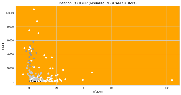
#Visualize clusters: Random Feature Pair-2 (inflation vs gdpp)import matplotlib.pyplot as plt_3plt_3.figure(figsize=(12,6))plt_3.scatter(datacopy[‘inflation’],datacopy[‘gdpp’],c=db.labels_) plt_3.title(‘Inflation vs GDPP (Visualize DBSCAN Clusters)’, fontsize=15)plt_3.xlabel(“Inflation”, fontsize=12)plt_3.ylabel(“GDPP”, fontsize=12)plt_3.rcParams[‘axes.facecolor’] = ‘orange’plt_3.show()

＃可視化群集：隨機特征對2(通貨膨脹與gdpp)將matplotlib.pyplot導入為plt_3plt_3.figure(figsize =(12,6))plt_3.scatter(datacopy ['inflation']，datacopy ['gdpp']，c = db.labels_)plt_3.title('通貨膨脹與GDPP(可視化DBSCAN集群)'，字體大小= 15)plt_3.xlabel(“通貨膨脹”，字體大小= 12)plt_3.ylabel(“ GDPP”，字體大小= 12)plt_3。 rcParams ['axes.facecolor'] ='橙色'plt_3.show()

If you want to implement code from your hand then click the button and implement code end to end with explanation in brief.

如果您想用手執行代碼，請單擊按鈕并以簡短的說明從頭到尾實現代碼。

If u like to read this article and have common interest in similar projects then we can grow our network and can work for more real time projects.

如果您喜歡閱讀本文并且對類似項目有共同的興趣，那么我們可以擴大我們的網絡并可以從事更多實時項目。

For more details connect with me on my Linkedin account!

有關更多詳細信息，請通過我的Linkedin帳戶與我聯系！

THANKS!!!!

謝謝！！！！