in collaboration with Hsu Chung Chuan, Lin Min Htoo, and Quah Jia Yong.

與許忠傳，林敏濤和華佳勇合作。

1. Introduction

1.簡介

Since the early 1990s, several countries, mostly in the European Union and North America, had started to deregulate their traditionally state-controlled energy sectors[1,2]. This has resulted in the marketisation of energy where — like other commodities — energy is traded competitively in free markets, using instruments such as the spot and derivative contracts [3]. Unlike most commodities, however, energy load is strongly dependent on short-term environmental conditions such as temperature, wind speed, cloud cover, precipitation, et cetera, in addition to the intensity of day-to-day business activities. This dependency, compounded by the fact that energy is a non-storable commodity, makes energy load highly volatile.

自1990年代初以來，幾個國家(主要在歐盟和北美)已開始放松對傳統上由國家控制的能源部門的管制[1,2]。 這導致了能源的市場化，在該市場上，與其他大宗商品一樣，能源通過使用即期和衍生合約等工具在自由市場中競爭性交易[3]。 但是，與大多數商品不同，除了日常業務活動的強度外，能源負荷還強烈依賴于短期環境條件，例如溫度，風速，云量，降水等 。 這種依賴性，再加上能源是不可儲存的商品這一事實，使能源負荷極易波動。

The environmental dependence and volatility present a unique challenge to energy traders whose aim is to accurately predict energy production (commonly between 18 or 48 hours following the forecast)[4]. Recently, methods developed in machine learning, especially the Deep Neural Network (DNN), has shown impressive predictive performance in energy load forecasting tasks. We will review this briefly in Section 2. Despite their impressive performance, however, most of these methods only utilise common loss functions such as mean squared error (MSE), mean absolute error (MAE) and their variants e.g. root mean squared error (RMSE), relative root mean squared error (RRMSE) and mean absolute percentage errors (MAPE) [5,6,7,8,9]. This presents a limitation since these losses only minimise the difference between predicted and true values, which although convenient, often do not reflect the potentially intricate profit structure outlined by the specific set of contracts a trader agrees to.

環境依賴性和波動性對能源貿易商提出了獨特的挑戰，其目標是準確預測能源生產(通常在預測后的18或48小時之間)[4]。 最近，在機器學習中開發的方法，尤其是深度神經網絡(DNN)，在能源負荷預測任務中顯示出令人印象深刻的預測性能。 我們將在第2節中對此進行簡要回顧。盡管它們的性能令人印象深刻，但是大多數方法僅利用常見的損失函數，例如均方誤差(MSE)，均值絕對誤差(MAE)及其變量，例如均方根誤差(RMSE) )，相對均方根誤差(RRMSE)和平均絕對百分比誤差(MAPE)[5,6,7,8,9]。 由于這些損失只會使預測值與真實值之間的差異最小化，因此存在局限性，盡管這很方便，但通常無法反映出交易者同意的一組特定合同概述的潛在復雜的利潤結構。

Hence, we propose a loss we call the Opportunity Loss defined as the difference between the optimal reward of predicting exactly the true value and the reward of the estimate. This loss is thus flexible and follows the the profit structure outlined by a trader’s contract.

因此，我們提出了一種稱為機會損失的損失，定義為準確預測真實價值的最佳獎勵與估計的獎勵之間的差。 因此，這種損失是靈活的，并且遵循交易者合同概述的利潤結構。

We test our approach using hourly data from 8 wind farms in the Ile-de-France region between January 1st, 2017 to July 14th, 2020. The datasets are provided by Réseau de transport d'électricité and Terra Weather as part of the AI4Impact 2020 Datathon [10]. On several DNN architectures we show that our proposed loss performs comparably to common loss functions when profit structure is symmetric, however, outperforms common loss functions when profit structure is asymmetric. Remarkably, these performances are achieved without needing to pass variables used to calculate opportunity loss as model inputs.

我們使用2017年1月1日至2020年7月14日之間法蘭西島地區的8個風電場的每小時數據測試我們的方法。數據集由Réseaude transport d'électricité和Terra Weather作為AI4Impact 2020的一部分提供Datathon [10]。 在幾種DNN架構上，我們表明，當利潤結構對稱時，我們提出的損失與普通損失函數具有可比性，但是當利潤結構不對稱時，其損失優于常見損失函數。 值得注意的是， 無需將用于計算機會損失的變量作為模型輸入即可實現這些性能。

In addition to our proposed loss, we also introduce a novel way to jointly encode the effect of wind direction and speed which improves simulated trading performance. This is especially novel given that most studies consider only either wind speed or wind direction as features [11,12,13,14], but rarely both [15].

除了我們提出的損失外，我們還引入了一種新穎的方式來聯合編碼風向和風速的影響，從而改善了模擬交易的績效。 鑒于大多數研究僅將風速或風向視為特征[11,12,13,14]，而很少同時考慮兩者[15]，所以這是特別新穎的。

We segment this article into six sections. In the next section we explain the DNN and baseline architectures we consider for the experiments. Section 3 explains common losses and introduces our proposed opportunity loss. We then explain our experiment design, including our approach to feature engineering, in section 4. We present the results of our experiments in section 5, before concluding in section 6.

我們將本文分為六個部分。 在下一部分中，我們將解釋我們為實驗考慮的DNN和基線架構。 第3節介紹了常見的損失，并介紹了我們建議的機會損失。 然后，我們在第4節中說明我們的實驗設計，包括我們進行特征工程的方法。在第6節中總結之前，我們在第5節中介紹了我們的實驗結果。

2. Models

2.型號

Recent developments in energy load forecasting has seen impressive predictive performance of DNN architectures. Many have shown that DNNs outperform canonical time-series prediction models such as ARIMA [9, 16, 17] and Linear Models [18]. This article considers state-of-the art architectures that has recently been adopted for the energy production forecasting domain such as one-dimensional CNN (1D-CNN) [19,20], Long Short Term Memory (LSTM)[6,21,22], and LSTM-CNN combined architectures [5,7]. As baseline comparisons, we use the persistence and the Multi-Layer Perceptron (MLP).

能量負荷預測的最新發展已經看到了DNN架構令人印象深刻的預測性能。 許多研究表明，DNN的性能優于規范的時間序列預測模型，例如ARIMA [9，16，17]和線性模型[18]。 本文考慮了最近在能源生產預測領域采用的最新架構，例如一維CNN(1D-CNN)[19,20]，長期短期記憶(LSTM)[6,21， 22]和LSTM-CNN組合架構[5,7]。 作為基線比較，我們使用持久性和多層感知器(MLP)。

2.1. Persistence

2.1。 堅持不懈

Persistence is the simplest forecast model that we use here solely for evaluation purposes. It assumes that the energy production after the prediction window L is the same as the production when the prediction is made. It can be described in equation as:

持久性是我們僅用于評估目的的最簡單的預測模型。 假設在預測窗口L之后的能量產生與進行預測時的能量相同。 可以用等式描述為：

2.2. MLP

2.2。 MLP

The MLP is an architecture inspired by the interaction between neurons in the human brain. Each unit of the MLP is described as a linear combination between the input a with learnable weights W and a bias b which is then transformed by a non-linear activation function σ(·). An example of a non-linear activation function is the rectified linear unit (ReLU) which transforms all negative values to zero and leaves all positive values unchanged.

MLP是受人腦神經元之間相互作用啟發的架構。 MLP的每個單位被描述為具有可學習權重W的輸入a和偏置b之間的線性組合，然后通過非線性激活函數σ( · )對其進行轉換 。 非線性激活函數的一個示例是整流線性單位(ReLU)，它將所有負值都轉換為零，而使所有正值保持不變。

Using these units as building blocks one can build a network that reroutes the information from inputs X into the estimate y_hat, essentially creating a network that can be thought as an approximation of a non-linear function f(X) [23]. Below is an example of an MLP with three hidden layers with widths five, four, and three.

使用這些單元作為構建塊，可以構建一個網絡，該網絡將信息從輸入X重新路由到估計值y_hat ，從本質上創建一個網絡，可以將其視為非線性函數f(X)的近似值[23]。 下面是一個MLP的示例，該MLP具有三個隱藏層，其寬度分別為5、4和3。

2.3. CNN

2.3。 有線電視新聞網

The Convolutional Neural Network (CNN) was originally developed in its two dimensional flavour by [25], which has since been popular in field of image recognition owing to its high degree of invariance to deformations such as translation and scaling [26]. That said, this architecture has also been recently adopted in its one-dimensional form to model time-series as illustrated in [27] and [28].

卷積神經網絡(CNN)最初是由[25]以其二維形式開發的，由于其對變形(例如平移和縮放)的高度不變性，此后在圖像識別領域廣受歡迎[26]。 也就是說，這種架構最近也以其一維形式被采用來建模時間序列，如[27]和[28]所示。

A 1D-CNN is built of two kinds of layer, the convolutional layer and the maxpool layer. The convolution layer is a function that takes in a sequence of data and outputs a sequence of convolutions with less than or equal the original length. A convolution operation with kernel size k linearly combines k data with learnable weights W and bias b. A convolution layer of kernel size k and stride s, thus, convolves the first k data in a sequence before sliding across by s steps and convolving next k data. This repeats until the kernel reaches the end of the sequence.

1D-CNN由兩種層構成：卷積層和maxpool層。 卷積層是一種功能，該功能接受一系列數據并輸出小于或等于原始長度的一系列卷積。 內核大小為k的卷積運算將k個數據與可學習的權重W和偏差b線性組合。 因此，內核大小為k且步幅為s的卷積層在序列中對前k個數據進行卷積，然后滑動s步并對下一個k數據進行卷積。 重復此過程，直到內核到達序列末尾為止。

A maxpool layer of kernel size k and stride s does the same operation as the convolutional layer, but instead of convolving the data together, it takes the maximum value of the k data. Once the input has passed through both layers, the output is activated by a non-linear function σ(·), just like in the MLP.

內核大小為k且步幅為s的maxpool層執行與卷積層相同的操作，但不是將數據卷積在一起，而是取k個數據的最大值。 輸入經過兩層后，就可以通過非線性函數σ( · )激活輸出，就像在MLP中一樣。

In practice, 1D-CNN architectures have several convolution-maxpool layers stacked on top of one another which then is connected to a fully-connected (MLP) layer which generates the estimate.

在實踐中，一維CNN架構具有幾個彼此疊置的卷積最大池層，然后將它們連接到生成估計值的全連接(MLP)層。

2.4. LSTM

2.4。 LSTM

Besides CNNs, another popular neural network architecture for forecasting is the Recurrent Neural Network (RNN). The RNN architecture as shown in Figure 3.a below has a recurrent property, which means that the input to a hidden layer h_t is not only the data X_t (like in MLP), but also the output of the previous hidden layer h_{t-1}. This property allows the network to encode temporal patterns.

除了CNN，另一種流行的用于預測的神經網絡架構是遞歸神經網絡(RNN)。 如下圖3.a所示的RNN架構具有循環屬性，這意味著隱藏層h_t的輸入不僅是數據X_t (如MLP中一樣)，而且是前一個隱藏層h_ {t的輸出-1} 。 此屬性允許網絡對時間模式進行編碼。

LSTM [29] is a popular enhancement to the RNNs as shown in Figure 3.b, which operations are illustrated by:

LSTM [29]是RNN的一種流行增強，如圖3.b所示，其操作如下所示：

In these equations, f_t, i_t, and o_t are the forget, input and output gates which are identified by the weights W_f, W_i, W_o and biases b_f, b_i, b_o respectively. Whilst, C_t, C{tilde}_t denote the cell state and proposal cell state, and W_c, b_c are cell weights and biases, respectively. In this case σ(·) denotes the sigmoid activation function and tanh(·) denotes the hyperbolic tangent activation function.

在這些等式中，F_噸，I_T，和 O_t同是忘記，其通過權重W_f，W_i，W_o和偏見b_f識別的輸入和輸出門，b_i，分別b_o。 雖然，C_ 噸 ，C {波浪} _ t指小區狀態和建議細胞狀態，并且W_ C，分別b_c是細胞重量和偏見。 在這種情況下， σ( · )表示S型激活函數，而tanh(·)表示雙曲正切激活函數。

In application, the forget and input gates collectively learn to keep essential information the past into the cell state and to forget useless ones. The output gate learns the conditions at which the information in the cell state is relevant to the next hidden state. This enhancement allows the neural network to remember important information from a distant past which vanilla RNNs struggle with due to vanishing gradients. Like CNNs, the last hidden state is usually passed through a fully connected layer to obtain the estimate.

在應用中，忘記門和輸入門共同學習如何將過去的重要信息保持在單元狀態，并忘記無用的信息。 輸出門學習單元狀態中的信息與下一個隱藏狀態相關的條件。 這種增強使神經網絡可以記住遠距離的重要信息，而過去的香草由于梯度的消失而難以與之聯系。 像CNN一樣，最后的隱藏狀態通常會經過一個完全連接的層以獲得估計。

2.5. LSTM-CNN Combination

2.5。 LSTM-CNN組合

Following [7], we also tried a combination of the two architectures which they claim to capture local and temporal trends simultaneously. Their architecture firstly runs one LSTM and one CNN simultaneously on the model inputs, which outputs are then concatenated before it is passed through a fully connected layer. This is illustrated below in Figure 4.

按照[7]，我們還嘗試了兩種架構的組合，他們聲稱可以同時捕獲本地和時間趨勢。 他們的體系結構首先在模型輸入上同時運行一個LSTM和一個CNN，然后在輸出通過完全連接的層之前對其進行串聯。 如下圖4所示。

3. Loss

3.損失

Models described in Section 2 learn their parameters through minimisation of a loss function. In regression tasks, losses commonly reflect the difference between the actual value to be predicted and the estimate. Once defined, we can backpropagate [30] the loss gradient through the layers, updating the parameters along the way.

第2節中描述的模型通過最小化損失函數來學習其參數。 在回歸任務中，損失通常反映了要預測的實際值與估計值之間的差異。 定義好之后，我們可以反向傳播[30]穿過各層的損耗梯度，并一路更新參數。

3.1. Common Losses

3.1。 常見損失

One of the most common loss functions for forecasting is the mean square error (MSE) defined as

用于預測的最常見損失函數之一是均方誤差(MSE)，其定義為

Another common loss function is the mean absolute error (MAE) defined as

另一個常見的損??失函數是平均絕對誤差(MAE)，定義為

which is often used when robustness to outliers is a concern.

當需要考慮對異常值的魯棒性時，通常會使用它。

3.2. Opportunity Loss

3.2。 機會損失

While the previously mentioned losses and their variants are good for its mathematical tractability and simplicity, in application these losses can be limiting. For instance, the profit structure defined by a set of contracts agreed by a trader can be asymmetric where traders must pay a higher penalty for overprediction as compared to underprediction (in the form of opportunity cost). In this example, MSE and MAE cannot capture accurately this asymmetric profit structure.

盡管前面提到的損耗及其變體在數學上的易處理性和簡單性方面都很不錯，但在應用中這些損耗可能是有限的。 例如，由交易者達成的一組合同定義的利潤結構可能是不對稱的，與相對于預測不足(以機會成本的形式)相比，交易者必須為預測過度付出更高的懲罰。 在此示例中，MSE和MAE無法準確捕獲這種不對稱的利潤結構。

Given the possibility of intricate profit structures with many variables and interactions, instead of using the common losses we propose implementing the opportunity loss defined as

鑒于而是采用我們提出實現定義為機會損失的共同損失諸多變數和交互復雜的利益結構的可能性，

where Rbar{(S)}_n is the optimal revenue (i.e. perfect forecast) and Rhat{(S)}_n is the estimated revenue, both calculated with respect to the profit structure S. This creates a flexible loss that can describe any revenue structure given that the revenue is optimal when predictions are perfect. We will show that our proposed loss performs better than MSE and MAE for some revenue structures even when some of the inputs defining the loss is not a feature the neural network is trained on.

其中Rbar {(S)} _ n是最佳收入(即完美的預測)， Rhat {(S)} _ n是估計收入，兩者都是針對利潤結構S進行計算的 。 假設預測完美時收益是最優的，這將產生一個可以描述任何收益結構的靈活虧損。 我們將證明，即使某些定義損失的輸入不是神經網絡所訓練的特征，我們提出的損失在某些收入結構上也比MSE和MAE更好。

4. Experiments

4.實驗

4.1. Dataset description

4.1。 數據集描述

In our experiments, we use aggregated hourly wind energy production data of wind farms in the Ile-de-France region as provided by Réseau de transport d’électricité’s online database [31] which is illustrated in Figure 6. In addition to wind energy, we also use hourly wind speed (m/s) and direction (degrees North) data from 8 wind farms in Ile-de-France provided by Terra Weather as additional predictors. The later dataset is provided as part of the AI4impact Datathon [10]. Both datasets span the period between January 1st, 2017 to July 14th, 2020, which is the period we use for this study.

在我們的實驗中，我們使用了法蘭西島大區風電場的每小時風能發電總量數據，該數據由Réseaude transport d'électricité的在線數據庫[31]提供，如圖6所示。我們還使用了Terra Weather提供的來自法蘭西島上8個風電場的每小時風速(m / s)和風向(北度)數據作為其他預測指標。 后來的數據集作為AI4impact Datathon [10]的一部分提供。 這兩個數據集的時間跨度為2017年1月1日至2020年7月14日，這是我們用于本研究的時間段。

As some wind farms only start operations within the period stated above, we impute the values prior to a farm’s starting date with zeros. Then, we linearly interpolate the remaining missing datapoints. Time and wind-related features as mentioned in the next subsection are then added to this dataset.

由于某些風電場僅在上述期限內開始運營，因此我們將在風電場開始日期之前的值估算為零。 然后，我們線性插值剩余的缺失數據點。 然后，將在下一部分中提到的與時間和風有關的特征添加到該數據集中。

We normalise the data and measure the differences in wind energy production between each timepoint before reorganising the data into prediction windows of size 64 which will be used to predict change in wind energy 18 hours later. In doing this we aim to predict the differences between energy production at a time point and the energy production 18 hours later.

我們將數據標準化并測量每個時間點之間風能產生的差異，然后將數據重新組織到大小為64的預測窗口中，該窗口將用于預測18小時后的風能變化。 為此，我們旨在預測某個時間點的能量生產與18小時后的能量生產之間的差異 。

Lastly, we split the dataset into training, validation, and testing sets with 24,608 rows, 3,076 rows, and 3,076 rows respectively.

最后，我們將數據集分為訓練集，驗證集和測試集，分別具有24,608行，3,076行和3,076行。

4.2. Feature Engineering

4.2。 特征工程

To model this data, we engineer features from common predictors of wind energy production, namely time, wind speed, and wind direction. In this subsection we explain three feature engineering approaches. These approaches are implemented on top of common forecasting features such as difference, momentum, force, mean, median, kurtosis, et cetera. We present a detailed list of experiments we ran with different features in Supplementary Materials 1.

為了對這些數據進行建模，我們設計了風能生產的常見預測變量的特征，即時間，風速和風向。 在本小節中，我們解釋了三種特征工程方法。 這些方法是在常見的預測特征(例如差異，動量，力，均值，中位數，峰度等)之上實現的 。 我們提供了補充材料1中具有不同功能的實驗的詳細清單。

4.2.1. Time

4.2.1。 時間

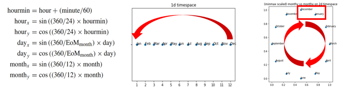
Time can be an important feature in wind energy forecasting as it may encode information about time-sensitive patterns as well as periodicity. In this article we consider two representation of time, one dimensional time and two dimensional time.

時間可能是風能預測中的重要特征，因為它可以對有關時間敏感模式以及周期性的信息進行編碼。 在本文中，我們考慮時間的兩種表示形式，即一維時間和二維時間。

One dimensional time encodes the time elapsed since the first observation which is implemented by adding the index of the time series as a feature. This may improve performance by providing the information allowing the model to learn about possible long-term trends that changes over time.

一維時間編碼自第一次觀察以來經過的時間，這是通過將時間序列的索引添加為特征來實現的。 通過提供允許模型學習隨時間變化的可能的長期趨勢的信息，可以提高性能。

Two dimensional time, on the other hand, can be used to represent periodicity. This is implemented as a trigonometric transformation [32, 33] described in Figure 7.

另一方面，二維時間可以用來表示周期性。 這被實現為圖7中描述的三角變換[32，33]。

4.2.2. Wind direction

4.2.2。 風向

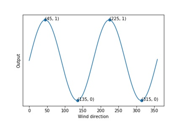
Like time, wind direction (often given in degrees North) is also cyclical. Hence, we also designed a trigonometric transformation, describing the direction with

像時間一樣，風向(通常以北度為單位)也是周期性的。 因此，我們還設計了一個三角變換，用

instead of degrees, where α is the wind direction.

而不是度，其中α是風向。

As shown in Figure 8, this transformation improves (Pearson’s) correlation between wind direction and energy production. We conjecture that including these more correlated features as model inputs may help improve model performance.

如圖8所示，此變換改善了風向與能量產生之間的(皮爾遜氏)相關性。 我們推測，將這些更相關的功能作為模型輸入包括在內可能有助于提高模型性能。

4.2.3. Joint effect encoding of wind speed and direction

4.2.3。 風速和風向的聯合效果編碼

As illustrated in Figure 9, wind speed alone is not directly correlated to energy output. Wind direction also plays a role since if the wind is not blowing at an optimal direction, despite high wind speed, energy production can be small. We hypothesise that wind blowing perpendicular to the turbines would not be able to turn it, resulting in zero or very little production.

如圖9所示，僅風速并不與能量輸出直接相關。 風向也起著重要作用，因為盡管風速很高，但如果風向不是最佳方向吹動，則能量產生會很小。 我們假設垂直于渦輪機的風將無法使其轉動，從而導致零產量或非常少的產量。

From Figure 9, a scatterplot of energy production against wind direction in one of the largest wind farms, we noted two distinct clusters. The first cluster is centred around 45 degrees North, and the second at 225 degrees North, which is at the same axis but blowing in the opposite direction. We noted that the closer the wind direction to this axis, the higher the wind energy production (illustrated as darker red spots). Thus, we inferred that ideal direction for the wind turbines is around 45 and 225 degrees North. Conversely, we also hypothesise from Figure 9 that the direction that minimises energy production is at 135 and 315 degrees North.

從圖9可以看出，在最大的風電場之一中，能源生產相對于風向的散布圖顯示了兩個不同的集群。 第一個星團的中心大約是北緯45度，第二個星團的中心是北緯225度，它的軸線相同，但方向相反。 我們注意到，風向越靠近此軸，風能產生就越高(如圖中暗點所示)。 因此，我們推斷出風力渦輪機的理想方向大約為北45度和225度。 相反，我們也從圖9假設，使能量產生最小化的方向是在135度和315度以北。

We thus devised a novel function to capture the joint effect of wind speed and direction described in this trigonometric output function

因此，我們設計了一個新穎的函數來捕獲此三角輸出函數中描述的風速和風向的聯合效應

where offset is the ideal wind direction. By multiplying speed with the trigonometric transformation of the direction, we get an overall function that considers both ideal wind direction and wind speed. As shown in Figure 11, this feature is better correlated with wind energy production.

其中偏移是理想的風向。 通過將速度乘以方向的三角變換，我們得到一個既考慮理想風向又考慮風速的整體函數。 如圖11所示，此功能與風能生產更好地關聯。

4.3. Model Parameters

4.3。 型號參數

Every DNN models takes a time series sequence of length 64 x d, where d is the feature dimension which varies according to the experiment. Our implementation of the MLP model consists of 4 hidden layers with widths 1024, 512, 256 and 128. Our 1D-CNN model is implemented with 4 convolutional layers having 64, 128, 256, and 512 channels with kernel sizes of 9, 7, 5, and 3 and maxpool layer of size 2. The last output of the convolutional layer is then passed through a fully connected layer of size 512. The LSTM model is implemented with 128 hidden and cell nodes each and a fully connected layer of size 512. The CNN-LSTM hybrid uses the hyperparameters above with a fully connected layer of 512.

每個DNN模型都采用長度為64 x d的時間序列，其中d是隨實驗變化的特征維。 我們的MLP模型實現包含4個隱藏層，寬度分別為1024、512、256和128。我們的1D-CNN模型由4個卷積層實現，這些卷積層具有64、128、256和512個通道，內核大小分別為9、7， 5、3和maxpool層的大小為2。然后，卷積層的最后輸出通過大小為512的完全連接層。LSTM模型是通過128個隱藏節點和單元節點以及大小為512的完全連接層實現的CNN-LSTM混合體使用上面的超參數以及512個完全連接的層。

For all the models described in the previous paragraph, we run 20 epochs with batch size of 256, using 0.001 learning rate, 0.1 dropout and early stopping with patience 2 and minimum permissible decrease in validation loss is 0.00005 smaller than the existing minimum. We use the ReLU activation for all nodes in these models.

對于上一段所述的所有模型，我們以0.001的學習率，0.1的輟學率和耐心2盡早停止運行了20個時期，批次大小為256，驗證損失的最小允許減少量比現有最小值減少了0.00005。 我們將ReLU激活用于這些模型中的所有節點。

We implement our models in PyTorch 1.5.0 which codes are available at https://github.com/kristoforusbryant/energy_production_forecasting/.

我們在PyTorch 1.5.0中實現了我們的模型，其代碼可從https://github.com/kristoforusbryant/energy_production_forecasting/獲得 。

4.4. Trading Simulation

4.4。 交易模擬

To assess trading performances of our models against varying profit structures, we use a simple deterministic simulation model defined by starting cash-in-hand (CIH) balance b_0, overprediction penalty o per unit, revenue of r per unit, and debt penalty d per unit.

為了評估針對不同利潤結構的模型的交易性能，我們使用簡單的確定性模擬模型，該模型通過啟動手頭現金(CIH)余額b_0，每單位的過高預測罰款o，每單位r的收入和每單位r的債務罰款d定義 。單元。

Starting with a balance of b_0, for every prediction made, if the model predicts less than the true value, r is credited per unit of prediction to the total balance b. For example, assume r = 10 cents/kWh, and the forecasted energy is 90kWh while actual energy produced is 100kWh. One then earns 90*10= 900 cents. The extra 10kWh can be thought as opportunity cost that one could have earned but did not.

從余額b_0開始，對于每個預測，如果模型預測的值小于真實值，則每預測單位將r記入總余額b 。 例如，假設r = 10 cents / kWh ，則預測能量為90kWh，而實際產生的能量為100kWh。 然后一個人賺90 * 10 = 900美分。 額外的10kWh可以認為是一個人本可以賺取但沒有的機會成本。

On the other hand, if prediction is more than the true value, r is credited per unit of true value, but o is deducted per unit of overprediction. For example, assume further that o = 20 cents/kWh, and the forecasted energy is 90kWh while actual energy produced is 80kWh. Then, one earns 80*10=800 cents from actual energy but pay 20*10=200 cents to spot the difference. Hence our net revenue is 800–200=600 cents.

另一方面，如果預測值大于真實值，則每單位真實值記入r值，但每單位過度預測則減去o值。 例如，進一步假設o = 20 cents / kWh ，預測的能量為90kWh，而實際產生的能量為80kWh。 然后，一個人從實際能量中賺取80 * 10 = 800美分，但支付20 * 10 = 200美分以發現差額。 因此，我們的凈收入是800-200 = 600美分。

Lastly, when balance less than or equal to zero, for every unit one overpredicts they must take on a loan which costs them d. For example, assume further that d = 100 cents/kWh. If the starting balance prior to the trade is 200 cents and one predicts 20 kWh when true output is 0 kWh, they are first penalised by 10 * 20 cents which brings their balance down to 0. In addition, they must take on a loan of 100*10 = 1,000 cents, which leaves them with a balance of -1,000 cents after the trade.

最后，當余額小于或等于零時，對于每個單位，人都高估了他們必須借入一筆貸款，從而使他們付出d的代價。 例如，進一步假設d = 100分/ kWh。 如果交易前的初始余額為200美分，并且當真實輸出為0 kWh時預測為20 kWh，則它們首先將受到10 * 20美分的罰款，這會使它們的余額降低到0。此外，他們還必須借入100 * 10 = 1,000美分，交易后剩下的余額為-1,000美分。

Our we experiment with two scenarios, namely the symmetric revenue structure where r = 10 and b = 10, and an asymmetric revenue structure where r = 10 and b = 50. In both cases, the starting balance b_0 = 10,000,000 and d = 100. We test these two scenarios with our CNN-LSTM model using MSE, MAE and opportunity loss defined according to the simulation.

我們在兩種情況下進行實驗，即r = 10和b = 10的對稱收入結構，以及r = 10和b = 50的非對稱收入結構。 在兩種情況下，初始余額b_0 = 10,000,000和d = 100 。 我們使用根據模擬定義的MSE，MAE和機會損失，使用CNN-LSTM模型測試了這兩種情況。

5. Results

5.結果

In this section we present the results to our experiments. All values showing standard deviations are the means of 10 repeats and all trading simulations are ran with the starting balance b_0=10,000,000.

在本節中，我們將結果介紹給我們的實驗。 所有顯示標準差的值都是10次重復的平均值，并且所有交易模擬均以初始余額b_0 = 10,000,000進行。

5.1. CNN and LSTM based models outperform baselines

5.1。 基于CNN和LSTM的模型優于基準

As shown in Figures 12.a and Table 1, the 1D-CNN and LSTM based models perform significantly better than baselines MLP and persistence in both MSE loss and simulation performance. Among the CNN and LSTM models, vanilla LSTM architecture does slightly better, obtaining the best simulation profit of 52.5 (0.21) and MSE of 0.01386(.00228). CNN and CNN-LSTM combined performance are comparable with this result as shown in Table 1. The MLP, although performs poorer than the more advanced DNNs, still perform significantly better than persistence.

如圖12.a和表1所示，基于1D-CNN和LSTM的模型的性能明顯優于基線MLP，并且在MSE損失和仿真性能方面都具有持久性。 在CNN和LSTM模型中，香草LSTM架構的性能稍好一些，獲得了52.5(0.21)的最佳模擬利潤和0.01386(.00228)的MSE。 如表1所示，CNN和CNN-LSTM的綜合性能可與該結果相媲美。盡管MLP的性能比更高級的DNN差，但其性能仍遠優于持久性。

A similar trend is observed with the lagged (Pearson’s) correlations between the prediction and the target. As Figure 12.b and Table 1 shows, 1D-CNN, LSTM and CNN-LSTM hybrid have peak correlations at time 0. This is in contrast with MLP’s peak correlation that is lagged by 18 hours. Among the former methods, CNN, LSTM an CNN-LSTM hybrid has comparable peak correlation values with the LSTM model having highest peak correlation.

預測和目標之間的滯后(皮爾遜)相關性觀察到類似的趨勢。 如圖12.b和表1所示，一維CNN，LSTM和CNN-LSTM混合體在時間0處具有峰值相關性。這與MLP的峰值相關性滯后18小時相反。 在以前的方法中，CNN，LSTM和CNN-LSTM混合體具有可比的峰值相關值，而LSTM模型具有最高的峰值相關性。

5.2. Opportunity loss improves simulation performance with asymmetric revenue structures

5.2。 機會損失通過不對稱的收入結構提高了仿真性能

Figure 14.a shows the first experiment with symmetric revenue structure. Given the symmetric structure, we see that simulation performance of the three losses are comparable with MSE, MAE and opportunity loss earning 5.16(.11), 5.16(.08), 5.18(.16), respectively.

圖14.a顯示了第一個采用對稱收入結構的實驗。 給定對稱結構，我們看到這三種損失的模擬表現分別與MSE，MAE和機會損失可比，分別為5.16(.11)，5.16(.08)，5.18(.16)。

When tested with an asymmetric revenue structure, however, the opportunity loss performs significantly better than the MAE and MSE losses with 3.87(.23), 3.40(.66), 2.92(.79) as seen from Figure 14.b. Between the common losses, MAE does significantly better than MSE.

然而，當使用非對稱收入結構進行測試時，機會損失的表現明顯優于MAE和MSE損失，其收益分別為3.87(.23)，3.40(.66)，2.92(.79)，如圖14.b所示。 在常見損失之間，MAE的表現明顯優于MSE。

This result is to be expected as MSE and MAE losses are unaware of the asymmetric revenue structure it is simulated on. That said, it is noteworthy that the opportunity loss still performs well despite some of its constituents not taken as model inputs. In this simulation, for instance, the initial balance and the balance history used to calculate the opportunity loss are not inputs to the model, yet the neural networks can still show improved performance. Not needing to have all the parameters that defines the loss as model inputs makes the model more flexible, which may be helpful with cases where profit structures changes over time.

由于MSE和MAE虧損并未意識到其模擬的不對稱收入結構，因此可以預期這一結果。 就是說，值得注意的是，盡管機會損失仍然是表現良好的，但其中一些因素并未作為模型輸入。 例如，在此仿真中，用于計算機會損失的初始余額和余額歷史記錄未輸入模型，但神經網絡仍可以顯示出改進的性能。 不需要將定義損失的所有參數都作為模型輸入，可以使模型更加靈活，這在利潤結構隨時間變化的情況下可能會有所幫助。

As Figure 15 shows, compared to the model trained with MSE, those trained with asymmetric opportunity loss tend to underpredict more than to overpredict. The tendency to be more conservative in their predictions while still keeping a tight variance around the actual difference is a possible explanation to why models trained on asymmetric opportunity loss outperforms those trained on MSE.

如圖15所示，與通過MSE訓練的模型相比，那些通過非對稱機會損失訓練的模型傾向于低估而不是高估。 他們的預測趨于保守的趨勢，同時仍使實際差異保持緊密變化，這可能解釋了為什么在非對稱機會損失下訓練的模型優于在MSE上訓練的模型。

5.3. Product of cosines-squared embedding improves performance

5.3。 余弦平方嵌入的乘積可提高性能

Table 3 illustrates the result of our feature engineering approaches on test loss (MSE) and simulation performance ran only on our CNN-LSTM architecture, but we expect comparable results from our LSTM and 1D-CNN architectures. Note that this table is the result of a semi-manual semi-greedy search on the space of feature sets. This means that as one goes down the row, features that improves performance is kept when running the next additional features.

表3展示了我們的功能測試方法在測試損失(MSE)和仿真性能上僅在我們的CNN-LSTM架構上運行的結果，但是我們希望LSTM和1D-CNN架構具有可比的結果。 請注意，此表是對要素集空間進行半手動半貪婪搜索的結果。 這意味著，隨著性能的提高，運行下一個附加功能時會保留提高性能的功能。

Table 3 first illustrate how the 2D time feature as explained in 4.2.1 does not improve performance. While this seems to be at odds with the results by [32, 33], we conjecture that this might be caused by the minimal autocorrelation of the wind energy production as illustrated in Figure 16. This figure shows only one peak at the start but no peak afterwards. This implies that periodic trend for this dataset is minimum, which might explain why the 2D time feature does not improve performance.

表3首先說明了4.2.1中說明的2D時間功能如何不會提高性能。 盡管這似乎與[32，33]的結果不一致，但我們推測這可能是由風能產生的最小自相關引起的，如圖16所示。該圖在開始時僅顯示一個峰值，但沒有之后達到頂峰。 這意味著此數據集的周期性趨勢是最小的，這可能可以解釋為什么2D時間功能無法改善性能。

We also observe that feature sets that includes first and second order differences improve performance, this seems to indicate that the way energy production, wind speed and wind direction changes is informative to forecasting the actual values of energy production.

我們還觀察到，包含一階和二階差異的特征集可提高性能，這似乎表明，能源生產，風速和風向變化的方式對于預測能源生產的實際價值具有指導意義。

Lastly, we also observe that our novel approach to encoding the joint effect between wind speed and direction as a trigonometric function (4.2.3) significantly improve prediction performance. A list of experiments we ran is detailed in Supplementary Material 1.

最后，我們還觀察到，我們將風速和風向之間的聯合效應編碼為三角函數(4.2.3)的新穎方法顯著提高了預測性能。 補充材料1中詳細列出了我們運行的實驗清單。

6. Discussion and Conclusion

6.討論與結論

In this article, we propose opportunity loss, a loss function that can be adapted to intricate profit structures. We prove in our simple asymmetry simulation that our loss function outperforms other losses in terms of the revenue earned. Further studies can consider implementing this approach on a more realistic simulations with more complex profit structures.

在本文中，我們提出機會損失，這是一種可以適應復雜的利潤結構的損失函數。 我們通過簡單的不對稱模擬證明，就收入而言，我們的損失函數優于其他損失。 進一步的研究可以考慮在具有更復雜的利潤結構的更現實的模擬中實施這種方法。

Remarkably, opportunity loss allows neural network models to learn the desired behaviour even when variables defining the loss function (such as initial balance) are not inputs to the model. We suspect this phenomenon might be caused by the neural networks implicitly learning latent representations of these loss variables, which is a possibility since they are the model inputs are not independent to the loss inputs. Further research can explore the extent to which — in terms of number of variables and independence– this observation holds.

值得注意的是，機會損失使神經網絡模型，甚至學習所需的行為時定義的損失函數(如初始余額)變量不輸入到模型中。 我們懷疑這種現象可能是由于神經網絡隱式學習了這些損失變量的潛在表示而引起的，這是有可能的，因為它們是模型輸入并不獨立于損失輸入。 進一步的研究可以探索這種觀察在多大程度上和獨立性方面。

Moreover, further analysis on the amount of data needed for training is interesting. We claim this because in energy load forecasting, contracts can change by the day or even sometimes by the hour, thereby continually changing the profit structure. Suppose that we have a flexible enough loss function such as the opportunity loss, the bottleneck for deployment of a truly flexible loss function lies in the amount of training needed to adjust the model to fit new loss functions.

此外，對培訓所需的數據量進行進一步分析很有趣。 我們之所以這樣說，是因為在能源負荷預測中，合同可能一天甚至一天都發生變化，從而不斷改變利潤結構。 假設我們具有足夠靈活的損失函數(例如機會損失)，則部署真正靈活的損失函數的瓶頸在于調整模型以適應新的損失函數所需的訓練量。

A tangential idea is to implement the idea from cooperative inverse reinforcement learning [34] which instead of defining the loss function analytically, makes the model learn its own loss function through manual feedback by humans. This process creates a neural representation of the loss function which may help in the case where profit structure is difficult to define analytically.

一個切線的想法是從協作逆強化學習中實現這個想法[34]，而不是通過分析定義損失函數，而是使模型通過人工反饋來學習自己的損失函數。 此過程創建了損失函數的神經表示，這在難以通過分析定義利潤結構的情況下可能會有所幫助。

Besides opportunity loss, we also implemented a novel encoding for the joint effect of wind speed and energy, which we have shown to improve performance.

除了機會損失之外，我們還針對風速和能量的聯合效應實施了一種新穎的編碼，已證明可以提高性能。

7. References

7.參考

[1] Watkiss, J. D., & Smith, D. W. (1993). The Energy Policy Act of 1992-A watershed for competition in the wholesale power market. Yale J. on Reg., 10, 447.

[1] Watkiss，JD，＆Smith，DW(1993)。 1992年的《能源政策法》-成為電力批發市場競爭的分水嶺。 耶魯J. ，10，447。

[2] Pollitt, M. G. (2019). The European single market in electricity: an economic assessment. Review of Industrial Organization, 55(1), 63–87.

[2] Pollitt，MG(2019)。 歐洲電力單一市場：經濟評估。 工業組織評論 ， 55 (1)，63–87。

[3] Bunn, D. W. (2004). Modelling prices in competitive electricity markets.

[3] Bunn，DW(2004)。 在競爭激烈的電力市場中對價格進行建模。

[4] https://energyanalyst.co.uk/an-introduction-to-electricity-price-forecasting/

[4] https://energyanalyst.co.uk/an-introduction-to-electricity-price-forecasting/

[5] Kuo, P. H., & Huang, C. J. (2018). An electricity price forecasting model by hybrid structured deep neural networks. Sustainability, 10(4), 1280.

[5] Kuo，PH，＆Huang，CJ(2018)。 基于混合結構深度神經網絡的電價預測模型。 可持續性 ， 10 (4)，1280。

[6] Wang, S., Wang, X., Wang, S., & Wang, D. (2019). Bi-directional long short-term memory method based on attention mechanism and rolling update for short-term load forecasting. International Journal of Electrical Power & Energy Systems, 109, 470–479.

[6] Wang，S.，Wang X.，Wang，S.，＆Wang，D.(2019)。 基于注意力機制和滾動更新的雙向長短期記憶方法用于短期負荷預測。 國際期刊電力與能源系統 ，109，470-479 的 。

[7] Tian, C., Ma, J., Zhang, C., & Zhan, P. (2018). A deep neural network model for short-term load forecast based on long short-term memory network and convolutional neural network. Energies, 11(12), 3493.

[7]田成，馬俊，張成，詹占平(2018)。 基于長短期記憶網絡和卷積神經網絡的深度神經網絡短期負荷預測模型。 能量 ， 11 (12)，3493。

[8] Dalto, M., Matu?ko, J., & Va?ak, M. (2015, March). Deep neural networks for ultra-short-term wind forecasting. In 2015 IEEE International Conference on Industrial Technology (ICIT) (pp. 1657–1663). IEEE.

[8] Dalto，M.，Matu?ko，J.和Va?ak，M.(2015年3月)。 深度神經網絡可用于超短期風能預報。 2015年IEEE工業技術國際會議(ICIT) (第1657年至1663年)。 IEEE。

[9] Ryu, S., Noh, J., & Kim, H. (2017). Deep neural network based demand side short term load forecasting. Energies, 10(1), 3.

[9] Ryu，S.，Noh，J.和Kim，H.(2017)。 基于深度神經網絡的需求側短期負荷預測。 能量 ， 10 (1)，3。

[10] https://ai4impact.org/dld.html

[10] https://ai4impact.org/dld.html

[11] Celik, A. N., & Kolhe, M. (2013). Generalized feed-forward based method for wind energy prediction. Applied Energy, 101, 582–588.

[11] Celik，AN和Kolhe，M.(2013)。 基于廣義前饋的風能預測方法。 應用能源 ，101，582-588。

[12] Kramer, O., Gieseke, F., & Satzger, B. (2013). Wind energy prediction and monitoring with neural computation. Neurocomputing, 109, 84–93.

[12] Kramer，O.，Gieseke，F.，＆Satzger，B.(2013)。 風能預測和神經計算監測。 神經計算 ，109，84-93。

[13] Grassi, G., & Vecchio, P. (2010). Wind energy prediction using a two-hidden layer neural network. Communications in Nonlinear Science and Numerical Simulation, 15(9), 2262–2266.

[13] Grassi，G.和Vecchio，P.(2010)。 使用兩層神經網絡的風能預測。 非線性科學與數值模擬中的通信 ， 15 (9)，2262-2266。

[14] Zhu, Q., Chen, J., Zhu, L., Duan, X., & Liu, Y. (2018). Wind speed prediction with spatio–temporal correlation: A deep learning approach. Energies, 11(4), 705.

[14]朱強，陳健，朱林，段旭，劉柳(2018)。 具有時空相關性的風速預測：一種深度學習方法。 能源 ， 11 (4)，705。

[15] Parks, K., Wan, Y. H., Wiener, G., & Liu, Y. (2011). Wind energy forecasting: A collaboration of the National Center for Atmospheric Research (NCAR) and Xcel Energy (No. NREL/SR-5500–52233). National Renewable Energy Lab.(NREL), Golden, CO (United States).

[15] Parks，K.，Wan，YH，Wiener，G.，＆Liu，Y.(2011)。 風能預測：國家大氣研究中心(NCAR)和Xcel Energy(No. NREL / SR-5500–52233)的合作。 美國科羅拉多州戈爾登的國家可再生能源實驗室(NREL)。

[16] Shi, H., Xu, M., & Li, R. (2017). Deep learning for household load forecasting — A novel pooling deep RNN. IEEE Transactions on Smart Grid, 9(5), 5271–5280.

[16] Shi，H.，Xu，M.，＆Li，R.(2017)。 用于家庭負荷預測的深度學習-一種新穎的深度RNN池。 IEEE Transactions on Smart Grid ， 9 (5)，5271–5280。

[17] Cao, Q., Ewing, B. T., & Thompson, M. A. (2012). Forecasting wind speed with recurrent neural networks. European Journal of Operational Research, 221(1), 148–154.

[17] Cao Q.，Ewing，BT和Thompson，MA(2012)。 使用遞歸神經網絡預測風速。 歐洲運籌學雜志 ， 221 (1)，148–154。

[18] Sfetsos, A. (2000). A comparison of various forecasting techniques applied to mean hourly wind speed time series. Renewable energy, 21(1), 23–35.

[18] Sfetsos，A.(2000)。 應用于平均風速時間序列的各種預測技術的比較。 可再生能源 ， 21 (1)，23–35。

[19] Zhao, X., Jiang, N., Liu, J., Yu, D., & Chang, J. (2020). Short-term average wind speed and turbulent standard deviation forecasts based on one-dimensional convolutional neural network and the integrate method for probabilistic framework. Energy Conversion and Management, 203, 112239.

[19] Zhao X.，Jiang，N.，Liu，J.，Yu，D.，＆Chang，J.(2020)。 基于一維卷積神經網絡和概率框架集成方法的短期平均風速和湍流標準差預測。 能源轉換和管理 ，203，112239。

[20] Kim, J., Moon, J., Hwang, E., & Kang, P. (2019). Recurrent inception convolution neural network for multi short-term load forecasting. Energy and Buildings, 194, 328–341.

[20] Kim，J.，Moon，J.，Hwang，E.，＆Kang，P.(2019)。 遞歸初始卷積神經網絡用于多短期負荷預測。 能源與建筑 ，194，328-341。

[21] Hu, Y. L., & Chen, L. (2018). A nonlinear hybrid wind speed forecasting model using LSTM network, hysteretic ELM and Differential Evolution algorithm. Energy conversion and management, 173, 123–142.

[21]胡亞蘭，陳陳(2018)。 基于LSTM網絡，滯回ELM和差分進化算法的非線性混合風速預測模型。 能源轉換和管理 ，173，123-142。

[22] Gensler, A., Henze, J., Sick, B., & Raabe, N. (2016, October). Deep Learning for solar power forecasting — An approach using AutoEncoder and LSTM Neural Networks. In 2016 IEEE international conference on systems, man, and cybernetics (SMC) (pp. 002858–002865). IEEE.

[22] Gensler，A.，Henze，J.，Sick，B.，和Raabe，N.(2016年10月)。 太陽能預測的深度學習-一種使用AutoEncoder和LSTM神經網絡的方法。 在2016年IEEE系統，人與控制論(SMC)國際會議上 (pp。002858–002865)。 IEEE。

[23] Goodfellow, I., Bengio, Y., & Courville, A. (2016). Deep learning. MIT press.

[23] I. Goodfellow，Y。Bengio和A. Courville，(2016年)。 深度學習 。 麻省理工學院出版社。

[24] https://developer.oracle.com/databases/neural-network-machine-learning.html

[24] https://developer.oracle.com/databases/neural-network-machine-learning.html

[25] Fukushima, K. (1988). Neocognitron: A hierarchical neural network capable of visual pattern recognition. Neural networks, 1(2), 119–130.

[25] Fukushima，K。(1988)。 Neocognitron：能夠視覺模式識別的分層神經網絡。 神經網絡 ， 1 (2)，119–130。

[26] LeCun, Y., Kavukcuoglu, K., & Farabet, C. (2010, May). Convolutional networks and applications in vision. In Proceedings of 2010 IEEE international symposium on circuits and systems (pp. 253–256). IEEE.

[26] LeCun，Y.，Kavukcuoglu，K.和Farabet，C.(2010年5月)。 卷積網絡及其在視覺中的應用。 在2010 IEEE會議論文集的電路和系統國際研討會上 (第253-256頁)。 IEEE。

[27] Oord, A. V. D., Dieleman, S., Zen, H., Simonyan, K., Vinyals, O., Graves, A., … & Kavukcuoglu, K. (2016). Wavenet: A generative model for raw audio. arXiv preprint arXiv:1609.03499.

[27] Oord, AVD, Dieleman, S., Zen, H., Simonyan, K., Vinyals, O., Graves, A., … & Kavukcuoglu, K. (2016). Wavenet: A generative model for raw audio. arXiv preprint arXiv:1609.03499 .

[28] Alves, T., Laender, A., Veloso, A., & Ziviani, N. (2018, December). Dynamic prediction of icu mortality risk using domain adaptation. In 2018 IEEE International Conference on Big Data (Big Data) (pp. 1328–1336). IEEE.

[28] Alves, T., Laender, A., Veloso, A., & Ziviani, N. (2018, December). Dynamic prediction of icu mortality risk using domain adaptation. In 2018 IEEE International Conference on Big Data (Big Data) (pp. 1328–1336). IEEE.

[29] Gers, F. A., Schmidhuber, J., & Cummins, F. (1999). Learning to forget: Continual prediction with LSTM.

[29] Gers, FA, Schmidhuber, J., & Cummins, F. (1999). Learning to forget: Continual prediction with LSTM.

[30] Goodfellow, I., Bengio, Y., & Courville, A. (2016). Deep learning. MIT press.

[30] Goodfellow, I., Bengio, Y., & Courville, A. (2016). Deep learning . MIT press.

[31] https://www.rte-france.com/en/eco2mix/eco2mix-telechargement-en

[31] https://www.rte-france.com/en/eco2mix/eco2mix-telechargement-en

[32] Moon, J., Park, S., Rho, S., & Hwang, E. (2019). A comparative analysis of artificial neural network architectures for building energy consumption forecasting. International Journal of Distributed Sensor Networks, 15(9), 1550147719877616.

[32] Moon, J., Park, S., Rho, S., & Hwang, E. (2019). A comparative analysis of artificial neural network architectures for building energy consumption forecasting. International Journal of Distributed Sensor Networks , 15 (9), 1550147719877616.

[33] https://medium.com/@linminhtoo/forecasting-energy-consumption-using-neural-networks-xgboost-2032b6e6f7e2

[33] https://medium.com/@linminhtoo/forecasting-energy-consumption-using-neural-networks-xgboost-2032b6e6f7e2

[34] Hadfield-Menell, D., Russell, S. J., Abbeel, P., & Dragan, A. (2016). Cooperative inverse reinforcement learning. In Advances in neural information processing systems (pp. 3909–3917).

[34] Hadfield-Menell, D., Russell, SJ, Abbeel, P., & Dragan, A. (2016). Cooperative inverse reinforcement learning. In Advances in neural information processing systems (pp. 3909–3917).

Supplementary Materials

Supplementary Materials

Supplementary materials can be found here: https://github.com/kristoforusbryant/energy_production_forecasting/.

Supplementary materials can be found here: https://github.com/kristoforusbryant/energy_production_forecasting/ .