As I promised in the previous article, Principal Component Analysis (PCA) with Scikit-learn, today, I’ll discuss the mathematics behind the principal component analysis by manually executing the algorithm using the powerful numpy and pandas libraries. This will help you to understand how PCA really works behind the scenes.

正如我在上一篇文章Scikit-learn中的主成分分析(PCA)中所承諾的那樣，今天，我將通過使用功能強大的numpy和pandas庫手動執行算法來討論主成分分析背后的數學原理。 這將幫助您了解PCA在幕后的工作原理。

Before proceeding to read this one, I highly recommend you to read the following article:

在繼續閱讀此文章之前，我強烈建議您閱讀以下文章：

• Principal Component Analysis (PCA) with Scikit-learn

  使用Scikit學習的主成分分析(PCA)

This is because this article is continued from the above article.

這是因為本文是上述文章的續篇。

In this article, I first review some statistical and mathematical concepts which are required to execute the PCA calculations.

在本文中，我首先回顧一些執行PCA計算所需的統計和數學概念。

PCA背后的統計概念 (Statistical concepts behind PCA)

意思 (Mean)

The mean (also called the average) is calculated by simply adding all the values and dividing by the number of values.

平均值 (也稱為平均值 )是通過簡單地將所有值相加并除以值的數量來計算的。

標準偏差 (Standard Deviation)

The standard deviation is a measure of how much of the data lies within proximity to the mean. It is the square root of the variance.

標準偏差是多少數據位于平均值附近的度量。 它是方差的平方根。

協方差 (Covariance)

The standard deviation is calculated on a single variable. The covariance is the variance of one variable against another. When the covariance of a variable is computed against itself, the result is the same as simply calculating the variance for that variable.

標準偏差是根據單個變量計算的。 協方差是一個變量相對于另一個變量的方差。 當針對自身計算變量的協方差時，結果與簡單地計算該變量的方差相同。

協方差矩陣 (Covariance Matrix)

A covariance matrix is a matrix representation of the possible covariance values that can be computed for all features of a dataset. It is required to execute the PCA of a dataset. The following image shows such a covariance matrix of a dataset which has 3 variables called X, Y and Z.

協方差矩陣是可以為數據集的所有特征計算的可能協方差值的矩陣表示。 需要執行數據集的PCA。 下圖顯示了這樣的數據集的協方差矩陣，該數據集具有3個變量，分別為X ， Y和Z。

cov(Y, X) is the covariance of Y with respect to X. It is same as the cov(X, Y). The diagonal elements of the covariance matrix give you the values of variance for each variable. For example, cov(X, X) is the variance of X.

cov(Y，X)是Y相對于X的協方差。 與cov(X，Y)相同 。 協方差矩陣的對角元素為您提供每個變量的方差值。 例如，COV(X，X)是X的方差。

A large value of the covariance of one variable against another would suggest that one feature changes significantly with respect to the other while a value close to zero would signify a very little change.

一個變量相對于另一個變量的協方差值較大將表明一個特征相對于另一個特征發生了顯著變化，而接近零的值表示變化很小。

To calculate the covariance matrix for a given dataset, we can use numpy cov() function or pandas DataFrame cov() method.

要計算給定數據集的協方差矩陣，我們可以使用numpy cov()函數或pandas DataFrame cov()方法。

PCA背后的數學概念 (Mathematical concepts behind PCA)

特征值和特征向量 (Eigenvalues and Eigenvectors)

Let A be an n x n matrix. A scalar λ is called an eigenvalue of A if there is a non-zero vector x satisfying the following equation:

設A為nxn矩陣 。 如果存在一個滿足以下等式的非零向量x ，則標量λ稱為A的特征值 ：

The vector x is called the eigenvector of A corresponding to λ.

向量x稱為與λ對應的A的特征向量 。

The above equation implicitly represents PCA. The following equation which is same as the above equation (but with different terms) directly represents PCA.

上述方程式隱含表示PCA。 以下公式與上面的公式相同(但術語不同)直接代表PCA。

Where,

哪里，

• A is an n x n square matrix. In terms of PCA, A is the covariance matrix.

  A是一個nxn方陣 。 就PCA而言， A是協方差矩陣。

• Σ represents all the eigenvalues in the form of a diagonal matrix which has the diagonal elements representing eigenvalues. The amount of variability within the dataset is indicated by the corresponding eigenvalue. This is done by describing how much contribution each eigenvector provides to the dataset. The larger the eigenvalue, the greater its contribution.

  Σ以對角矩陣的形式表示所有特征值，其中對角元素表示特征值。 數據集內的變化量由相應的特征值指示。 這是通過描述每個特征向量對數據集的貢獻來完成的。 特征值越大，貢獻越大。

• U represents all the eigenvectors in the form of an n x n square matrix.

  U以nxn方陣的形式表示所有特征向量。

We have discussed some statistical and mathematical concepts behind PCA. In the next steps, we calculate the eigenvalues and eigenvectors using the covariance matrix of the breast_cancer dataset. Then we perform the PCA. For the entire PCA process, we will only use numpy and pandas libraries and will not use the scikit-learn library except for the feature scaling.

我們討論了PCA背后的一些統計和數學概念。 在接下來的步驟中，我們將使用breast_cancer數據集的協方差矩陣來計算特征值和特征向量。 然后我們執行PCA。 對于整個PCA流程，除了功能擴展外，我們將僅使用numpy和pandas庫，而不使用scikit-learn庫。

使用numpy和pandas手動執行PCA (Execute PCA manually using numpy and pandas)

步驟1：導入庫并設置圖樣式 (Step 1: Import libraries and set plot styles)

As the first step, we import various Python libraries which are useful for our data analysis, data visualization, calculation and model building tasks. When importing those libraries, we use the following conventions.

第一步，我們導入各種Python庫，這些庫對于我們的數據分析，數據可視化，計算和模型構建任務很有用。 導入這些庫時，我們使用以下約定。

步驟2：獲取并準備數據 (Step 2: Get and prepare data)

The dataset that we use here is available in Scikit-learn. But it is not in the correct format that we want. So, we have to do some manipulations to get the dataset ready for our task. First, we load the dataset using Scikit-learn load_breast_cancer() function. Then, we convert the data into a pandas DataFrame which is the format we are familiar with.

我們在這里使用的數據集可以在Scikit-learn中找到。 但這不是我們想要的正確格式。 因此，我們必須進行一些操作才能使數據集為我們的任務做好準備。 首先，我們使用Scikit-learn load_breast_cancer()函數加載數據集。 然后，我們將數據轉換為我們熟悉的pandas DataFrame格式。

Now, the variable df contains a pandas DataFrame of the breast_cancer dataset. We can see its first 5 rows by calling the head() method. The following image shows a part of the dataset.

現在，變量df包含breast_cancer數據集的pandas DataFrame。 我們可以通過調用head()方法查看其前5行。 下圖顯示了數據集的一部分。

The full dataset contains 30 columns and 569 observations.

完整的數據集包含30列和569個觀察值。

步驟3： 獲取特征矩陣 (Step 3: Obtain the feature matrix)

The feature matrix contains the values of all 30 features in the dataset. It is a 569x30 two-dimensional Numpy array. It is stored in the X variable.

特征矩陣包含數據集中所有30個特征的值。 這是一個569x30的二維Numpy數組。 它存儲在X變量中。

步驟4：如有必要，對功能進行標準化 (Step 4: Standardize the features if necessary)

You can see that the values of the dataset are not equally scaled. So, we need to apply z-score standardization to get all features into the same scale. For this, we use Scikit-learn StandardScaler() class which is in the preprocessing submodule in Scikit-learn.

您會看到數據集的值沒有按比例縮放。 因此，我們需要應用z分數標準化，以使所有功能達到相同的比例。 為此，我們使用Scikit-learn StandardScaler()類，該類位于Scikit-learn的預處理子模塊中。

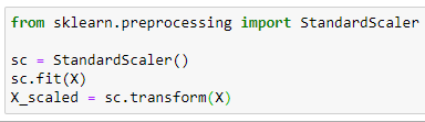
First, we import the StandardScaler() class. Then, we create an object of that class and store it in the variable sc. Then we use the sc object’s fit() method with the input X (feature matrix). This will calculate the mean and standard deviation for each variable in the dataset. Finally, we do the transformation with the transform() method of the sc object. The transformed (scaled) values of X are stored in the variable X_scaled which is also a 569x30 two-dimensional Numpy array.

首先，我們導入StandardScaler()類。 然后，我們創建該類的對象并將其存儲在變量sc中 。 然后，將sc對象的fit()方法與輸入X (功能矩陣)一起使用。 這將計算數據集中每個變量的平均值和標準偏差。 最后，我們使用sc對象的transform()方法進行轉換 。 X的轉換(縮放)值存儲在變量X_scaled中 ，該變量也為 569x30二維Numpy數組。

步驟5：計算協方差矩陣 (Step 5: Compute the covariance matrix)

Now, we compute the covariance matrix for all features of our dataset. Note that we use X_scaled matrix, not the X. To calculate the covariance matrix for our dataset, we can use numpy cov() function. We need to take the transpose of X_scaled because the covariance matrix is based on the number of features (30), not observations (569).

現在，我們為數據集的所有特征計算協方差矩陣。 請注意，我們使用X_scaled矩陣，而不是X。 要為我們的數據集計算協方差矩陣，我們可以使用numpy cov()函數。 我們需要對X_scaled進行轉置，因為協方差矩陣基于特征的數量(30)，而不是觀察值(569)。

The covariance matrix of our dataset is a 30x30 2d numpy array.

我們的數據集的協方差矩陣是30x30 2d numpy數組。

步驟6：計算協方差矩陣的特征值和特征向量 (Step 6: Compute the eigenvalues and eigenvectors of the covariance matrix)

We can use the eig() function to calculate the eigenvalues and eigenvectors of the covariance matrix. The eig() function is in the linalg module which is a subpackage of the numpy library.

我們可以使用eig()函數來計算協方差矩陣的特征值和特征向量。 在EIG()函數是linalg模塊這是numpy的庫的一個子包英寸

The variable eigenvalues returns all the eigenvalues.

變量特征值返回所有特征值。

The variable eigenvectors returns all the eigenvectors in the form of 30x30 2d numpy array.

變量特征向量以30x30 2d numpy數組的形式返回所有特征向量。

Then we get the transpose of eigenvectors.

然后我們得到特征向量的轉置。

The eigenvector for the first eigenvalue (13.304) is the first row of the eigenvectors array. It has 30 elements.

第一個特征值(13.304)的特征向量是特征向量數組的第一行。 它具有30個元素。

步驟7：從最高到最低對特征值和特征向量進行排序 (Step 7: Sort the eigenvalues and eigenvectors from the highest to the lowest)

About the first 20 eigenvalues were automatically sorted from the highest to the lowest. So, we do not need to sort the eigenvalues and eigenvectors. This is because we need just first 10 eigenvalues for our PCA process.

自動從最高到最低對大約前20個特征值進行排序。 因此，我們不需要對特征值和特征向量進行排序。 這是因為我們的PCA過程僅需要前10個特征值。

步驟8：將特征值計算為數據集中方差的百分比 (Step 8: Compute the eigenvalues as a percentage of the variance within the dataset)

From the above eigenvalues, we need only the first 10 eigenvalues to preserve 95.15% of the variability in the data. The corresponding (selected) eigenvectors for the first 10 eigenvalues are:

從以上特征值中，我們僅需要前10個特征值即可保留數據中95.15％的變異性。 前10個特征值的對應(選定)特征向量為：

步驟9：將縮放后的數據集乘以所選特征向量 (Step 9: Multiply the scaled dataset by the selected eigenvectors)

The dimensionality reduction process is a matrix multiplication of the selected eigenvectors and the (scaled) data to be transformed. Note that the transpose of the X_scaled is required to match the dimension when executing the matrix multiplication.

降維處理是所選特征向量與要轉換的(縮放)數據的矩陣相乘。 請注意，執行矩陣乘法時需要X_scaled的轉置以匹配尺寸。

Then we get the transpose of data_new matrix (2d array).

然后我們得到data_new矩陣(2d數組)的轉置。

Now the data_new array is in the right dimension. It contains the transformed data with 10 principal components.

現在， data_new數組的尺寸正確。 它包含具有10個主要成分的轉換數據。

步驟10：將轉換后的數據轉換成pandas DataFrame (Step 10: Convert transformed data into a pandas DataFrame)

Let’s create a pandas DataFrame using the values of all 10 principal components.

讓我們使用所有10個主要成分的值創建一個熊貓DataFrame。

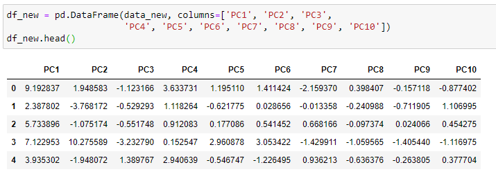
The transformed dataset now has 10 features (principal components) and 569 observations. The original dataset contains 30 features and 569 observations. Therefore, we have reduced the dimensionality of the data by 20 features preserving 95.15% of the variability in the data.

轉換后的數據集現在具有10個特征(主要成分)和569個觀測值。 原始數據集包含30個特征和569個觀測值。 因此，我們已通過減少20個要素的數據維數來保留了數據中95.15％的可變性。

步驟11：繪制主成分的值 (Step 11: Plot the values of the principal components)

The output is:

輸出為：

To verify, you can compare the results obtained here with the results obtained using the Scikit-learn PCA() by setting n_components=0.95. The results are exactly the same!

為了進行驗證，可以通過設置n_components = 0.95 ，將此處獲得的結果與使用Scikit-learn PCA()獲得的結果進行比較。 結果完全一樣！

Thank you for reading! See you in the next article.

感謝您的閱讀！ 下篇文章見。

This tutorial was designed and created by Rukshan Pramoditha, the Author of Data Science 365 Blog.

本教程設計和創造的Rukshan Pramoditha ，的作者數據科學365博客 。

本教程中使用的技術 (Technologies used in this tutorial)

• Python (High-level programming language)

  Python (高級編程語言)

• numPy (Numerical Python library)

  numPy (數字Python庫)

• pandas (Python data analysis and manipulation library)

  pandas (Python數據分析和操作庫)

• matplotlib (Python data visualization library)

  matplotlib (Python數據可視化庫)

• Jupyter Notebook (Integrated Development Environment)

  Jupyter Notebook (集成開發環境)

本教程中使用的統計概念 (Statistical concepts used in this tutorial)

• Mean

  意思

• Standard Deviation

  標準偏差

• Covariance

  協方差

• Covariance Matrix

  協方差矩陣

本教程中使用的數學概念 (Mathematical concepts used in this tutorial)

• Eigenvalues and Eigenvectors

  特征值和特征向量

• Matrix Multiplication

  矩陣乘法

• Matrix Transpose

  矩陣轉置

本教程中使用的機器學習 (Machine learning used in this tutorial)

• Principal Componnet Analysis (PCA)

  主成分分析(PCA)

2020–08–10

2020–08–10