用PYTHON探索數據 (EXPLORING DATA WITH PYTHON)

One of Tableau’s biggest advantages is how it lets you swim around in your data. You don’t always need a fine-tuned dashboard to find meaningful insights, so even someone with quite a basic understanding of Tableau can make a significant impact.

Tableau的最大優勢之一是它如何使您在數據中四處游蕩。 您不一定總是需要經過微調的儀表板才能找到有意義的見解，因此即使是對Tableau有了基本了解的人也可以產生重大影響。

For this article, we’ll play into that theme of not needing to know everything about a tool in order to build useful things with it. In our previous article, we touched on how you can create custom calculations and color visuals in Python to arrive at visuals that look quite similar to what we build in Tableau.

在本文中，我們將以不需要使用工具來構建有用的東西的所有知識為主題。 在上一篇文章中 ，我們談到了如何在Python中創建自定義計算和彩色視覺效果，從而獲得外觀與我們在Tableau中構建的外觀非常相似的視覺效果。

Today, let’s expand on what we’ve learned so far. Let’s see how we can take what we’ve seen up to this point and apply that to a common scenario: data exploration.

今天，讓我們擴展到目前為止所學的知識。 讓我們看看如何將到目前為止所看到的內容應用到一個常見的場景：數據探索。

搭建舞臺 (Setting the stage)

Previously, we took our ‘Sales’ and ‘Profit’ columns and created a new column named ‘Profit Ratio’. We then modified our plot from the first article, showing sales per product sub-category, and added color to the visual using our new ‘Profit Ratio’ metric:

以前，我們使用“銷售”和“利潤”列，并創建了一個名為“利潤率”的新列。 然后，我們從第一篇文章中修改了圖表，顯示了每個產品子類別的銷售額，并使用新的“利潤率”指標為視覺效果添加了顏色：

Whenever I teach a newcomer to Tableau how to use the software, I always plug in this visual somewhere in the mix.

每當我向Tableau教新手如何使用該軟件時，我總是將此視覺效果插入組合中的某個位置。

Something I view as a common mistake in data visualization is that people often think just because they can use color they always should. If we throw color randomly at our visuals, the results are typically no better than a simple table. Some visuals that get lost in the sauce can be downright confusing.

我認為數據可視化中的一個常見錯誤是，人們常常認為僅僅是因為他們可以使用他們應該經常使用的顏色。 如果我們在視覺上隨意扔顏色，結果通常不會比簡單表好。 醬汁中丟失的一些視覺效果可能會令人困惑。

In our use case, color is appropriate because it helps to quickly focus in on the desired “a-ha” revelation: higher volumes of sales do not necessarily lead to higher volumes of profits.

在我們的用例中，顏色是合適的，因為它有助于快速關注所需的“ ha-ha”啟示：更高的銷售量并不一定會帶來更高的利潤。

If this data were representative of a real business, a natural question that follows this visual might be: what’s happening that’s making some of our high-sale items less profitable (let’s assume this is bad) and some of our low-sale items highly profitable (let’s assume this is good)?

如果這些數據代表了真實的業務，那么視覺上的自然問題可能是：發生了什么事，這使我們的某些高價商品獲利能力下降(假設這是不好的)，而某些低價商品獲利率很高。 (假設這很好)？

To provide any meaningful answers to that question, we’re going to need to do a little data exploration.

為了提供對該問題的任何有意義的答案，我們將需要做一些數據探索。

步驟1：決定著眼于我們最具影響力的客戶 (Step 1: deciding to look at our most impactful customers)

First of all, context matters. The context of this data is that we are a retail store selling products. Customers can only buy what we sell, and they are buying at prices we have set. Therefore, if we have any negative profits this is a problem of our own making. Perhaps we are losing money on some products intentionally, lowering prices to attract customers whose other purchases make up for the initial loss.

首先，上下文很重要。 此數據的上下文是我們是一家銷售產品的零售商店。 客戶只能購買我們出售的產品，而他們是以我們設定的價格購買的。 因此，如果我們有任何負利潤，這是我們自己的問題。 也許我們故意在某些產品上虧本，降低價格以吸引其他購買來彌補最初損失的客戶。

My opinion is that regardless of what we discover, we want to land on something actionable. We need to be able to do something with the insights we generate, because otherwise what’s the point?

我的觀點是，無論我們發現什么，我們都希望找到可行的方法。 我們需要能夠做我們產生了一些見解，因為否則的話有什么意義？

So rather than analyze ALL of our customers, let’s focus in on our top customers. If you have a limited budget for outreach and customer service, it often makes sense to focus those resources on the top customers. For this exercise, let’s define our ‘top customers’ as those who spend the most money per order. Let’s keep it simple and say we’re interested in getting an overview of how the sales and profitability looks for our top 10% of customers.

因此，讓我們專注于主要客戶，而不是分析所有客戶。 如果您的宣傳和客戶服務預算有限，那么將這些資源集中在最重要的客戶上通常很有意義。 在本練習中，我們將“最大客戶”定義為每筆訂單花費最多的客戶。 讓我們保持簡單，說我們有興趣了解一下我們前10％的客戶的銷售和盈利能力概況。

For this Superstore data, that means we are looking at the top 159 customers.

對于此Superstore數據，這意味著我們正在尋找排名前159位的客戶。

步驟2：為客戶獲取每筆訂單的銷售額 (Step 2: getting the sales per order for our customers)

In Tableau, we would reach for a calculated field. In Python, we will want to first create a dataframe at the appropriate level of aggregation and then add a new column storing the average sales per order.

在Tableau中，我們將到達一個計算字段。 在Python中，我們將要首先在適當的聚合級別創建一個數據框，然后添加一個新列來存儲每個訂單的平均銷售額。

We want to know the sales per order for each customer, so the appropriate level of aggregation here is at the customer level (Customer ID).

我們想知道每個客戶的每個訂單的銷售額，因此此處適當的匯總級別是客戶級別(客戶ID)。

To calculate the sales per order for each customer, we will need to calculate the total sales and count the number of orders for each customer.

要計算每個客戶的每個訂單的銷售額，我們將需要計算總銷售額并計算每個客戶的訂單數量。

We can piece this together using a Pandas dataframe (note that ‘store_df’ is the dataframe storing all of the Superstore data):

我們可以使用Pandas數據框將其組合在一起(請注意，“ store_df”是存儲所有Superstore數據的數據框)：

orders_per_customer_df = store_df\
.groupby('Customer ID')\
.agg({
    'Order ID': pd.Series.nunique,
    'Sales': 'sum'
})\
.reset_index()\
.rename(columns={'Order ID': 'order_count'})\
.sort_values('Sales', ascending=False)

So let’s read through this line by line like it’s a book:

因此，讓我們像本書一樣逐行閱讀：

1. our output will be stored in a variable named ‘orders_per_customer_df’
   我們的輸出將存儲在名為“ orders_per_customer_df”的變量中
2. we are grouping our store data by the ‘Customer ID’ column
   我們正在按“客戶ID”列對商店數據進行分組
3. we are aggregating two columns; a unique count of ‘Order ID’ (represented by the pd.Series.nunique function)and the sum of ‘Sales’
   我們正在匯總兩列； “訂單ID”的唯一計數(由pd.Series.nunique函數表示)和“銷售”的總和
4. we are resetting the index of the resulting dataframe; if you have no idea what this means then try running the code without that statement and see how the results differ!
   我們正在重置結果數據幀的索引； 如果您不知道這意味著什么，請嘗試在不使用該語句的情況下運行代碼，然后看看結果有何不同！
5. we are renaming the ‘Order ID’ column to be ‘order_count’, which is a more appropriate name given we are no longer looking at the actual ID values
   我們將“訂單ID”列重命名為“ order_count”，這是一個更合適的名稱，因為我們不再查看實際的ID值
6. we are sorting the resulting dataframe by Sales, with highest values at the top
   我們將按Sales排序結果數據框，最高值在頂部

步驟3：計算每個客戶的每個訂單的總銷售額 (Step 3: calculate the total sales per order for each customer)

First, let’s admire a snippet of the dataframe we created in the previous step:

首先，讓我們欣賞上一步中創建的數據框的片段：

Alright, so we have a dataframe with our customers, the number of orders those customers made, and the total amount spent.

好了，因此我們擁有一個與客戶的數據框，這些客戶所下的訂單數量以及總花費。

To calculate the total sales per order, all we need to do is divide the ‘Sales’ column by the ‘order_count’ column.

要計算每個訂單的總銷售額，我們要做的就是將“銷售”列除以“ order_count”列。

orders_per_customer_df['avg_sales_per_order'] = \
orders_per_customer_df['Sales'] / orders_per_customer_df['order_count']

In the code snippet above, we have defined a new column ‘avg_sales_per_order’ and set that to be the result of our ‘Sales’ column divided by our ‘order_count’ column.

在上面的代碼段中，我們定義了一個新列“ avg_sales_per_order”，并將其設置為“銷售”列除以“ order_count”列的結果。

Here’s what that looks like, now sorted in descending order by ‘avg_sales_per_order’.

看起來像這樣，現在按降序按“ avg_sales_per_order”排序。

步驟4：查看訂單數分布 (Step 4: taking a look at the order count distribution)

Let’s do a quick side-quest. Comparing the order counts from the beginning of step 3 and the end of step 3, it seems there might be a lot of variation in the order counts of our customers.

讓我們做一個簡短的旁聽。 比較步驟3的開始和步驟3的結束之間的訂單數，看來我們客戶的訂單數可能會有很多差異。

In an effort to better understand customer behavior, let’s visualize the distribution of order counts.

為了更好地了解客戶行為，讓我們可視化訂單計數的分布。

sns.distplot(orders_per_customer_df['order_count'])

Running the line of code above gives us this:

運行上面的代碼行可以使我們做到這一點：

Ah, it looks like customers are naturally grouped into two camps. One group averages about 5 orders and the other averages about 25 orders.

嗯，看來客戶自然被分為兩個陣營。 一組平均約5個訂單，另一組平均約25個訂單。

This could be a reflection of our product mix; some customers may purchase a small amount of expensive items, while other customers shop more frequently for less expensive products.

這可能反映了我們的產品組合； 一些客戶可能會購買少量昂貴的商品，而其他客戶會更頻繁地購買價格較便宜的產品。

第4步：過濾數據以僅考慮前10％的客戶 (Step 4: filter our data to only consider the top 10% of customers)

In Tableau, one way to do this would be to create a filter for the ‘Customer ID’ field based on the calculated field for ‘avg_sales_per_order’ and only include the top 159 results.

在Tableau中，一種方法是基于“ avg_sales_per_order”的計算字段為“客戶ID”字段創建過濾器，并且僅包括前159個結果。

In Python, one potential solution is this:

在Python中，一種可能的解決方案是：

top_customers_df = \
store_df[store_df['Customer ID']\
.isin(orders_per_customer_df.head(159)['Customer ID'])]

Let’s dissect this.

讓我們對此進行剖析。

First of all, we are storing the results in a variable named ‘top_customers_df’.

首先，我們將結果存儲在名為“ top_customers_df”的變量中。

Second, we are using Pandas dataframe notation to essentially say “give us all rows of the ‘store_df’ dataframe that satisfy this condition.” In our case, the condition needing to be satisfied is that any given ‘Customer ID’ encountered must also be in the ‘Customer ID’ column for the top 159 rows of our ‘orders_per_customer_df’ dataframe.

其次，我們使用Pandas數據框表示法來表示“給我們滿足該條件的'store_df'數據框的所有行。” 在我們的情況下，需要滿足的條件是，遇到的任何給定“客戶ID”也必須位于“ orders_per_customer_df”數據幀的前159行的“客戶ID”列中。

In other words, we are filtering our store data such that we are only seeing data for the customer ID values seen in the top 159 rows of the dataframe that holds our top customers.

換句話說，我們正在過濾商店數據，以便只看到在擁有最大客戶的數據框的前159行中看到的客戶ID值的數據。

Go back and check out how we defined that ‘orders_per_customer_df’ dataframe if this is not clicking. Keep in mind that the .head(x) function returns the top x number of rows for any dataframe calling it.

返回并查看我們如何定義“ orders_per_customer_df”數據框(如果未單擊的話)。 請記住， .head(x)函數返回任何調用它的數據框的前x行數。

步驟5：預覽主要客戶的數據 (Step 5: preview the data for our top customers)

Now let’s take a quick look at the results, having filtered our store data to only include the top 159 customers. Let’s group this by ‘Sub-Category’ and aggregate the data to see total sales, average discount percentage, total profit, and the total number of orders.

現在，讓我們快速瀏覽一下結果，已篩選出商店數據，僅包括排名前159位的客戶。 讓我們按“子類別”將其分組并匯總數據以查看總銷售額，平均折扣率，總利潤和訂單總數。

subcat_top_customers_df = top_customers_df\
.groupby('Sub-Category')\
.agg({
    'Sales': 'sum',
    'Discount': 'mean',
    'Profit': 'sum',
    'Order ID': pd.Series.nunique
})\
.rename(columns={
    'Discount': 'Avg Discount',
    'Order ID': 'Num Orders'
})\
.sort_values('Profit', ascending=False)\
.reset_index()

Are you getting a feel for how these Pandas dataframes work? I recommend plugging the code in yourself and playing around with it. What happens if you change ‘sum’ to ‘median’, ‘min’, or ‘max’?

您對這些Pandas數據框的工作方式有感覺嗎？ 我建議您自己插入代碼并進行嘗試。 如果將“ sum”更改為“ median”，“ min”或“ max”會發生什么？

第6步：為前10％的客戶顯示結果 (Step 6: visualize the results for the top 10% of customers)

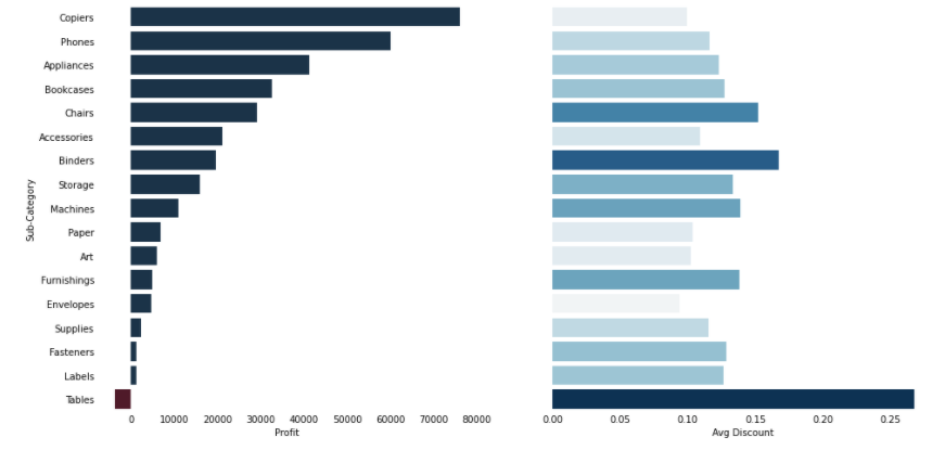
Before looking at the code to create this visual, let’s take a moment to soak it in. What are we looking at?

在查看創建視覺效果的代碼之前，讓我們花點時間將其浸入。我們在看什么？

On the left, we see total profits by sub-category. All of the bars where profits are above zero are colored blue. There is only one unprofitable sub-category here, and it’s ‘Tables’.

在左側，我們按子類別看到總利潤。 利潤高于零的所有條形都被涂成藍色。 這里只有一個無利可圖的子類別，它是“表格”。

Remember ‘Tables’ from the previous article? It was the sub-category screaming for attention. What’s interesting here is that Tables isn’t just unprofitable, it’s unprofitable even when looking at our top 10% of customers. Why is it unprofitable?

還記得上一篇文章中的“表格”嗎？ 這是子類別，引起人們的注意。 這里有趣的是，Tables不僅是無利可圖的，甚至在我們的前10％的客戶中也無利可圖。 為什么它無利可圖？

That’s where the visual on the right-hand side comes in highlighting the average discount. Once again, ‘Tables’ is screaming for attention, and here we can see that some abnormally high discounts are being given on our tables.

這就是右側視覺效果突出顯示平均折扣的地方。 再次，“桌子”尖叫著引起注意，在這里我們可以看到我們的桌子上有些異常高的折扣。

There may be a good business reason to heavily discount tables (perhaps it’s a loss leader), but at least now we know why tables are unprofitable: they are being discounted at >25%, which is much higher than any other product sub-category.

大量折扣表(也許是虧損的領先者)可能是一個很好的商業理由，但至少現在我們知道為什么該表無利可圖了：它們的折扣率> 25％，遠高于其他任何產品子類別。

第7步：了解視覺效果如何融合 (Step 7: understand how the visuals came together)

Here’s how the visual above works:

這是上面的視覺效果的工作方式：

fig, axs = plt.subplots(1, 2, figsize=(16, 8), sharey=True)sns.barplot(data=subcat_top_customers_df, 
            x='Profit', y='Sub-Category', ax=axs[0],
            palette=cm.RdBu(subcat_top_customers_df['Profit']), ci=False)sns.barplot(data=subcat_top_customers_df, 
            x='Avg Discount', y='Sub-Category', ax=axs[1],
            palette=cm.RdBu(subcat_top_customers_df['Avg Discount'] * 5.5), ci=False)axs[0].tick_params(axis='both', which='both', length=0)
axs[1].tick_params(axis='both', which='both', length=0)
axs[1].set_ylabel('')sns.despine(left=True, bottom=True)

The first line is something you’ll often see when working with Python plotting libraries. We are establishing a figure and a set of axes. The figure is like the canvas on which the visuals will live, and the axes act as the spine of our numerical and categorical data. In the first line we define a figure with 2 pieces of real estate: 1 row with two plots side by side. The ‘sharey’ parameter says that both visuals will share a y-axis, so there is no need to list out the sub-categories twice.

第一行是使用Python繪圖庫時經常看到的內容。 我們正在建立一個圖形和一組軸。 該圖就像是將在其上顯示視覺效果的畫布，并且軸是我們的數字和分類數據的脊柱。 在第一行中，我們定義了一個包含2個不動產的圖形：1行并排包含兩個地塊。 “ sharey”參數表示兩個視覺效果都將共享y軸，因此無需兩次列出子類別。

We then call on the Seaborn library, which was imported earlier under the alias ‘sns’, to plot our bar graphs. Here we define the dataframe providing our data, the columns which will provide our x-axis and y-axis, and the color gradient for each visual. The ‘ci’ parameter is set to ‘False’ to remove extra lines that would otherwise appear to show us confidence intervals. Go ahead and flip that to ‘True’ and see how the visual changes.

然后，我們調用Seaborn庫(該數據庫較早以別名“ sns”導入)來繪制條形圖。 在這里，我們定義了提供數據的數據框，將提供我們的x軸和y軸的列以及每個視覺圖像的顏色漸變。 “ ci”參數設置為“ False”以刪除多余的行，否則這些行似乎向我們顯示置信區間。 繼續并將其翻轉為“ True”，并查看外觀如何變化。

The final lines are cosmetic formatting, getting rid of tick marks and such. I highly recommend tinkering with this to get comfortable with the concept of formatting through code rather than through a click-and-drag interface like Tableau. Something nice about defining formatting through code is that you can build reusable functions that always apply your favorite formatting tricks.

最后一行是修飾格式，去除刻度線等。 我強烈建議對此進行修改，以使您熟悉通過代碼而不是通過諸如Tableau之類的單擊和拖動界面進行格式化的概念。 通過代碼定義格式的好處是，您可以構建可重用的功能，這些功能始終應用您喜歡的格式技巧。

Wrapping it up

結語

So, here we are. Our attention-seeking tables got the attention they wanted all along, and we got a bit more exposure to shaping and controlling our data using Pandas dataframes.

所以，我們到了。 我們的關注表一直吸引著他們一直想要的關注，而使用Pandas數據框來整形和控制數據的機會也更多了。

The data exploration here wasn’t earth-shattering, but if your comfortable with the Python code we’ve written up until now, then you’re ready to dive into our next session!

此處的數據探索并不是破天荒的事，但是如果您滿意我們到目前為止所編寫的Python代碼，那么您就可以開始進行下一個工作了！

Tune in next time, when we’ll explore joining data from different tables. Pandas makes this quite easy for us, so it’ll be a breeze for us to join our ‘Orders’ data to our ‘Returns’ data and answer the question: how many of our products have been returned? What percentage of our revenue is disappearing due to returns?

下次，當我們將探索來自不同表的聯接數據時，請進行調整。 熊貓對我們而言非常容易，因此將“訂單”數據與“退貨”數據結合起來并回答以下問題將是一件輕而易舉的事情：已經退回了多少產品？ 由于退貨，我們收入的百分之幾消失了嗎？

Hope to see you there!

希望在那里見到你！