My last articles tackled Bayes nets on quantum computers (read it here!), and k-means clustering, our first steps into the weird and wonderful world of quantum machine learning.

我的最后一篇文章討論了量子計算機上的貝葉斯網絡( 在這里閱讀！)和k-means聚類，這是我們進入量子機器學習的怪異世界的第一步。

This time, we’re going a little deeper into the rabbit hole and looking at how to build a neural network on a quantum computer.

這次，我們將更深入地研究兔子洞，并研究如何在量子計算機上構建神經網絡。

In case you aren’t up to speed on neural nets, don’t worry — we’re starting with neural nets 101.

如果您不適應神經網絡的速度，請不要擔心-我們將從神經網絡101開始。

什么是(經典的)神經網絡？ (What even is a (classical) neural network?)

Almost everyone has heard of neural networks — they’re used to run some of the coolest tech we have today — self driving cars, voice assistants, and even the software that generates super realistic pictures of famous people doing questionable things.

幾乎每個人都聽說過神經網絡-它們已經被用來運行我們今天擁有的一些最酷的技術-自動駕駛汽車，語音助手，甚至是生成可疑人物做事的超逼真的圖片的軟件。

What makes them different from regular algorithms is that instead of having to write down a set of rules, we need to provide networks with examples of the problem we want it to solve.

它們與常規算法的不同之處在于，我們不必編寫一組規則，而需要為網絡提供我們要解決的問題的示例。

We could feed a network with some data from the IRIS data set, which contains information about three kinds of flowers, and it might guess which kind of flower it is:

我們可以使用IRIS數據集中的一些數據為網絡提供數據，該數據包含有關三種花的信息，并且可能會猜測它是哪種花：

So now we know what neural networks do — but how do they do it?

所以現在我們知道了神經網絡的作用-但是它們是如何做到的？

重量，偏見和基石 (Weight, biases and building blocks)

Neural networks are made up of many small units called neurons, which look like this:

神經網絡由許多稱為神經元的小單元組成，如下所示：

Most neurons take multiple numeric inputs (the blue circles), and multiply each one of them by a weight (the w?s) that represent how important each input is. The larger the magnitude of a weight, the more important the associated input is.

大多數神經元接受多個數字輸入(藍色圓圈)，然后將每個數字與一個權重(w?s)相乘，代表每個輸入的重要性。 權重的大小越大，關聯的輸入就越重要。

The bias is treated like another weight, only that the input it multiplies always has a value of 1. When we add up all the weighted inputs, we get the activation value of the neuron, represented by the purple circle in the picture above:

偏差被視為另一個權重，只是它所乘的輸入始終具有一個值1。當我們將所有加權的輸入相加時，我們得到了神經元的激活值，由上圖中的紫色圓圈表示：

The activation value is then passed through a function (the blue rectangle), and the result is the output of the neuron:

激活值然后通過一個函數(藍色矩形)傳遞，結果是神經元的輸出：

We can change a neuron’s behavior by changing the function it uses to transform its activation value — for example, we could use a super simple transformation, like this one:

我們可以通過更改神經元用來轉換其激活值的函數來更改神經元的行為，例如，可以使用如下所示的超簡單轉換：

In practice, however, we use more complex ones, like the sigmoid function:

但是，實際上，我們使用更復雜的函數，例如Sigmoid函數：

How are neurons useful?

神經元有什么用？

They can make decisions based on the inputs they receive — for example, we could use a neuron to predict whether we’ll eat pizza or pasta the next time we eat out at an Italian place by feeding it the answers to three questions:

他們可以根據收到的輸入來做出決定-例如，我們可以使用神經元來預測下一次在意大利吃飯的時候是吃披薩還是面食，方法是將三個問題的答案提供給他們：

• Do I like the pasta at this restaurant?
  我喜歡這家餐廳的面食嗎？
• Does the restaurant have pesto sauce?
  該餐廳有香蒜醬嗎？
• Does the restaurant have a triple cheese pizza?
  這家餐廳有三層奶酪披薩嗎？

Putting aside possible health concerns, let’s see what the neuron might look like — we can encode the inputs using 0 to represent no, 1 to represent yes, and do the same with the outputs by mapping 0 and 1 to pasta and pizza respectively:

撇開可能的健康問題，讓我們看看神經元可能是什么樣子—我們可以使用0代表否，1代表是對輸入進行編碼，并通過分別將0和1映射到意大利面和披薩來對輸出進行相同的處理：

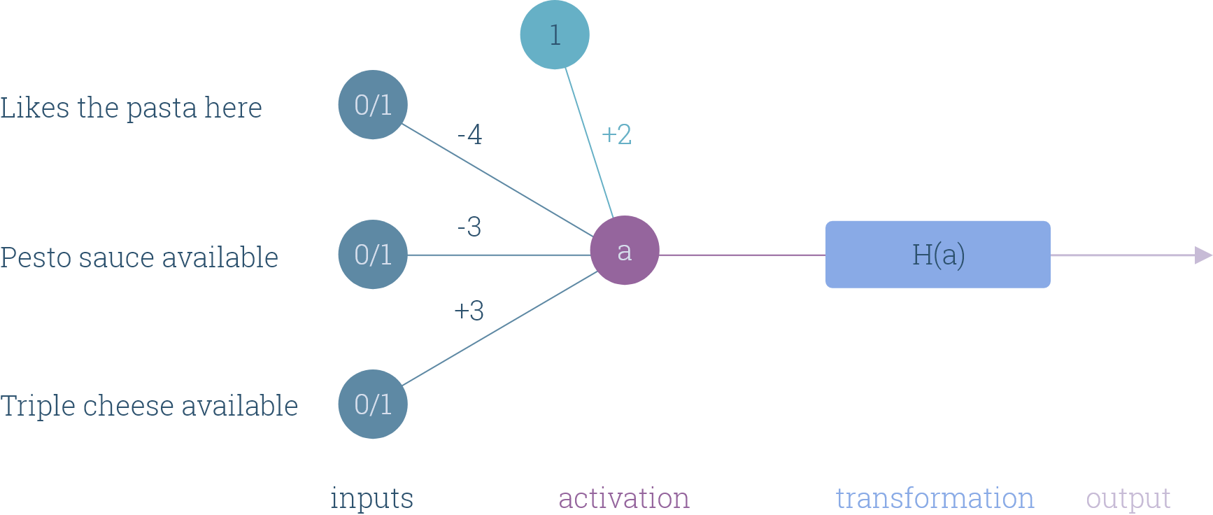
Let’s use the step function to transform the neuron’s activation value:

讓我們使用step函數來轉換神經元的激活值：

Just using one neuron, we can capture multiple decision making behaviours:

僅使用一個神經元，我們就可以捕獲多種決策行為：

• If we like the pasta at a restaurant, we choose to order pasta unless pesto sauce is out and they serve a triple cheese pizza.
  如果我們喜歡在餐廳吃意大利面，我們選擇點意大利面，除非沒有香蒜醬，并且可以提供三層奶酪比薩。
• If we don’t like the pasta at a restaurant, we order a pizza unless pesto sauce is available, and the triple cheese pizza is not.
  如果我們不喜歡在餐廳吃意大利面，我們會點披薩，除非有香蒜醬可用，而三層奶酪披薩則沒有。

We can also do things the other way — we can program a neuron so that it corresponds to a specific set of preferences.

我們還可以用其他方式來做事情-我們可以對神經元進行編程，使其與一組特定的偏好相對應。

If all we wanted to do was predict what we would eat the next time we go out, it would probably be easy to figure out a set of weights and biases for one neuron, but what if we had to do the same with a full-sized network?

如果我們要做的只是預測下次出門吃什么，可能很容易找出一組神經元的權重和偏見，但是如果我們必須對一個神經元做同樣的事情，那該怎么辦？規模的網絡？

It would probably take a while.

這可能需要一段時間。

Fortunately, instead of guessing the values of the weights we need, we can create algorithms that change the parameters of a network — the weights, biases, and even the structure — so that it can learn a solution for a problem we want to solve.

幸運的是，我們無需猜測所需的權重值，而是可以創建可更改網絡參數(權重，偏差甚至結構)的算法，以便它可以為我們要解決的問題學習解決方案。

下降到頂部 (Going down to get to the top)

Ideally, a network’s prediction would be the same as the label associated with the input we feed it — so the smaller the difference between the prediction and actual output, the better the set of weights the network has learned.

理想情況下，網絡的預測應與與我們為其輸入的輸入相關聯的標簽相同-因此，預測與實際輸出之間的差異越小，網絡所獲權重集就越好。

We quantify this difference using a loss function, which can take any form we want, like this one, which is called the quadratic loss function:

我們使用損失函數來量化這種差異，損失函數可以采用我們想要的任何形式，例如這種形式，稱為二次損失函數：

y(x) is the desired output and o(x, θ) is the network’s output when fed data x with parameters θ— since the loss is always non negative, once it takes on values close to 0, we know that the network has learned a good parameter set. Of course, there are other problems that can crop up, like over-fitting, but we’ll ignore those for now.

y(x)是期望的輸出，而o(x，θ)是在饋送帶有參數θ的數據x時網絡的輸出-由于損耗始終為非負值，一旦取值接近于0，我們就知道網絡具有學習了一個好的參數集。 當然，還會出現其他問題，例如過度擬合，但我們暫時將其忽略。

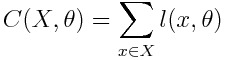
Using the loss function, we can figure out what the best parameter set for our network is:

使用損失函數，我們可以找出為我們的網絡設置的最佳參數是：

So instead of guessing weights, all we need to do is minimize C with respect to parameters θ — which we can do using a technique called gradient descent:

因此，除了猜測權重之外，我們要做的就是相對于參數θ最小化C ，我們可以使用稱為“梯度下降”的技術來做到這一點：

All we’re doing here is looking at how the loss changes if we increase the value of θ?, and then updating θ? so that the loss decreases by a little bit. η is a small number which controls by how much we change θ? every time we update it.

我們在這里所做的只是查看如果增加θ?的值后損耗如何變化，然后更新θ?以使損耗稍微降低。 η是一個很小的數字，它控制著每次更新θ?時會改變多少。

Why do we need η to be small? We could just adjust it so that the loss on the current x is close to zero after just one update— most times this is not a great idea, because while it would reduce the loss on the current x, it often leads to much worse performance on all the other data samples we feed to the network.

為什么我們需要η小？ 我們可以對其進行調整，以使一次更新后當前x的損失接近零-多數情況下，這不是一個好主意，因為雖然這會減少當前x的損失，但通常會導致更差的性能在所有其他數據樣本上，我們將其饋送到網絡。

Awesome!

太棒了！

Now that we’ve got the basics down, let’s figure out how to build a quantum neural network.

現在，我們已經掌握了基礎知識，接下來讓我們弄清楚如何構建量子神經網絡。

進入量子宇宙 (Into the quantumverse)

The quantum neural net we’ll be building doesn’t work the exact same way as the classical networks we’ve worked on so far—instead of using neurons with weights and biases, we encode the input data into a bunch of qubits, apply a sequence of quantum gates, and change the gate parameters to minimize a loss function:

我們將要建立的量子神經網絡的工作方式與迄今為止我們所研究的經典網絡完全不同-我們不是使用具有權重和偏差的神經元，而是將輸入數據編碼為一堆qubit，應用一系列量子門，并更改門參數以最小化損耗函數：

While that might sound new, the idea is still the same — change the parameter set to minimize the difference between the network predictions and input labels.

盡管這聽起來很新，但想法還是一樣的-更改參數集以最大程度地減少網絡預測和輸入標簽之間的差異。

To keep things simple, we’ll be building a binary classifier — meaning that every data point fed to the network has to have an associated label of either 0 or 1.

為簡單起見，我們將構建一個二進制分類器-這意味著饋入網絡的每個數據點都必須具有0或1的關聯標簽。

How does it work?

它是如何工作的？

We start by feeding some data x to the network, which is passed through a feature map — a function that transforms the input data into a form we can use to create the input quantum state:

我們首先將一些數據x饋入網絡，然后通過特征圖傳遞給網絡-該函數將輸入數據轉換為可用于創建輸入量子態的形式：

The feature map we use can look like almost anything — here’s one that takes in a two dimensional vector x, and spits out an angle:

我們使用的特征圖看起來幾乎可以是任何東西-這是一個輸入二維向量x并吐出一個角度的圖：

Once x is encoded as a quantum state, we apply a series of quantum gates:

將x編碼為量子態后，我們將應用一系列量子門：

The network output, which we’ll call π(x, θ), is the probability of the last qubit being measured as in the |1? state, plus a bias term that is added classically:

網絡輸出，我們稱之為π( x ， θ)是在| 1〉狀態下測量最后一個qubit的概率，加上經典添加的偏置項：

The Z? ? ? stands for a Z gate applied to the last qubit.

Z?代表施加到最后一個量子位的Z門。

Finally, we take the output and the label associated with x, and use them to compute the loss over the sample — we’ll use the same quadratic loss from above. The cost over the entire data set X we feed the network then becomes:

最后，我們獲取與x關聯的輸出和標簽，并使用它們來計算樣本的損失-我們將從上方使用相同的二次損失。 然后，我們為網絡提供的整個數據集X的成本變為：

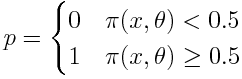
The prediction of the network p can be obtained from the output:

網絡p的預測可以從輸出中獲得：

Now all we need to do is to figure out how to compute the gradients of the loss function l(x, θ). While we could do it classically, that would be boring — what we need is a way to compute them on a quantum computer.

現在，我們要做的就是弄清楚如何計算損失函數l ( x ，θ)的梯度。 盡管我們可以經典地做到這一點，但這將很無聊–我們需要的是一種在量子計算機上進行計算的方法。

一種計算梯度的新方法 (A new way to compute gradients)

Let’s start by differentiating the loss function with respect to a parameter θ?:

讓我們從關于參數θ?的損耗函數開始：

Let’s expand the last term:

讓我們擴展最后一個術語：

We can quickly get rid of the constant terms — and in the case that θ? = b, we know that the gradient is simply 1:

我們可以快速擺脫常數項-并且在θ?= b的情況下，我們知道梯度只是1：

Now, using the product rule, we can expand further:

現在，使用乘積規則，我們可以進一步擴展：

That probably looks a little painful to read — but thanks to the Hermitian conjugate (the ?), this has a concise representation:

讀起來可能有點痛苦-但由于使用了Hermitian共軛(?)，因此表示簡潔：

Since U(θ) is made up of multiple gates, each of them controlled by a different parameter (or sets of parameters), finding the partial derivative of U only involves differentiating the gate U?(θ?) that is dependent on θ?:

由于U (θ)由多個門組成，每個門由不同的參數(或一組參數)控制，因此找到U的偏導數僅涉及區分門U? (θ?) 取決于θ?：

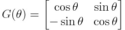
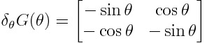
This is where the form we choose for each U? becomes important. We’ll use the same form for every U?, which we’ll call a G gate — the choice of form is arbitrary, so you could use any other form you can think of instead:

在這里，我們為每個U?選擇的形式變得很重要。 我們將對每個U?使用相同的形式，我們將其稱為G門-形式的選擇是任意的，因此您可以使用可以想到的任何其他形式來代替：

Now that we know what each U? looks like, we can find its derivative:

現在我們知道每個U?的樣子， 我們可以找到它的派生詞：

Lucky for us, we can express this in terms of the G gate:

對我們來說很幸運，我們可以用G來表示 門：

So all that’s left is to figure out how to create a circuit that gives us the inner product form we need:

因此，剩下的就是弄清楚如何創建一個電路，為我們提供所需的內部產品形式：

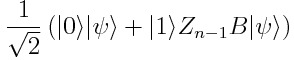
The easiest way to get a measurable that is proportional to this is to use the Hadamard test — first, we prepare the input quantum state and push an ancilla into superposition:

獲得與之成比例的可測量值的最簡單方法是使用Hadamard檢驗 -首先，我們準備輸入量子態并將輔助子項推入疊加狀態：

Now apply Z? ? ?B onto ψ, conditioned on the ancilla being in the 1 state:

現在，將Z?B?B應用于 ψ，條件是附加柱處于1狀態：

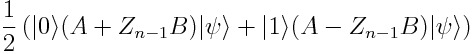
Then flip the ancilla, and do the same with A:

然后翻轉ancilla，并使用A進行相同操作：

Finally, apply another Hadamard gate onto the ancilla:

最后，將另一個Hadamard門應用到輔助部件上：

Now the probability of measuring the ancilla as 0 is

現在測量輔助線為0的概率為

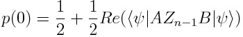
So if we substitute U(θ) for B, and a copy of U(θ) with U? swapped out for its derivative for A, then the probability of the ancilla qubit will give us the gradient of π(x, θ) with respect to θ?.

因此，如果我們用U (θ)代替B ，并且用U?的U (θ)的副本替換為A的導數， 那么輔助量子位的概率將給我們π( x ， 相對于θ?。

Great!

大！

We figured out a way to analytically compute gradients on a quantum computer — now all that’s left is to build our quantum neural network.

我們找到了一種在量子計算機上分析計算梯度的方法-現在剩下的就是建立我們的量子神經網絡。

建立量子神經網絡 (Building a quantum neural network)

Let’s import all the modules we need to kick things off:

讓我們導入所有需要啟動的模塊：

from qiskit import QuantumRegister, ClassicalRegister
from qiskit import Aer, execute, QuantumCircuit
from qiskit.extensions import UnitaryGate
import numpy as np

Now let’s take a look at some of our data (you can get it right here!) — it’s a processed version of the IRIS data set, with one class removed:

現在，讓我們看一些數據(您可以在這里找到它！)—它是IRIS數據集的處理后的版本，其中刪除了一個類：

0.803772773,0.5516087658,0.2206435063,0.0315205009,0
0.714141252,0.2664706164,0.6182118301,0.1918588438,1
0.7761140001,0.5497474167,0.3072117917,0.03233808334,0
0.8609385733,0.4400352708,0.2487155878,0.05739590488,0
0.690525124,0.3214513508,0.6071858849,0.2262065061,1

We need to separate the features (the first four columns) from the labels:

我們需要將功能(前四列)與標簽分開：

data = np.genfromtxt("processedIRISData.csv", delimiter=",")
X = data[:, 0:4]
features = np.array([convertDataToAngles(i) for i in X])
Y = data[:, -1]

Now let’s build a function that will do the feature mapping for us.

現在，讓我們構建一個為我們進行功能映射的函數。

Since the input vectors are normalized and 4 dimensional, there is a super simple option for the mapping — use 2 qubits to hold the encoded data, and use a mapping that just recreates the input vector as a quantum state.

由于輸入向量是歸一化的和4維的，因此映射有一個超級簡單的選擇-使用2個量子位來保存編碼數據，并使用僅將輸入向量重新創建為量子態的映射。

For this we need two functions — one to extract angles from the vectors:

為此，我們需要兩個函數-一個從向量中提取角度：

def convertDataToAngles(data):"""Takes in a normalised 4 dimensional vector and returns three angles such that the encodeData function returns a quantum state with the same amplitudes as the vector passed in. """prob1 = data[2] ** 2 + data[3] ** 2prob0 = 1 - prob1angle1 = 2 * np.arcsin(np.sqrt(prob1))prob1 = data[3] ** 2 / prob1angle2 = 2 * np.arcsin(np.sqrt(prob1))prob1 = data[1] ** 2 / prob0angle3 = 2 * np.arcsin(np.sqrt(prob1))return np.array([angle1, angle2, angle3])

Another to convert the angles we get into a quantum state:

另一種將角度轉換為量子態的方法：

def encodeData(qc, qreg, angles):"""Given a quantum register belonging to a quantumcircuit, performs a series of rotations and controlledrotations characterized by the angles parameter."""    qc.ry(angles[0], qreg[1])qc.cry(angles[1], qreg[1], qreg[0])qc.x(qreg[1])qc.cry(angles[2], qreg[1], qreg[0])qc.x(qreg[1])

This might seem a little confusing, but understanding how it works isn’t essential to building the QNN — you can read up on it here if you like.

這似乎有些令人困惑，但是了解它的工作方式對于構建QNN并不是必不可少的-如果愿意，可以在這里閱讀。

Now we can write the functions we need to implement U(θ), which will take the form of alternating layers of RY and CX gates.

現在我們可以編寫實現U (θ)所需的函數，該函數將采用RY和CX交替層的形式 蓋茨。

Why do we need the CX layers?

為什么我們需要CX層？

If we didn’t include them, we wouldn’t be able to perform any entanglement operations, which would limit the area within the Hilbert space that our network can reach — using CX gates, the network can capture interactions between qubits that it wouldn't be able to without them.

如果不包括它們，我們將無法執行任何糾纏操作，這將限制我們的網絡在希爾伯特空間內可以到達的區域-使用CX門，網絡可以捕獲量子比特之間的相互作用，不能沒有他們。

We’ll start with the G gates:

我們將從G門開始：

def GGate(qc, qreg, params):"""Given a parameter α, return a singlequbit gate of the form[cos(α), sin(α)][-sin(α), cos(α)]"""    u00 = np.cos(params[0])u01 = np.sin(params[0])gateLabel = "G({})".format(params[0])GGate = UnitaryGate(np.array([[u00, u01], [-u01, u00]]), label=gateLabel)return GGatedef GLayer(qc, qreg, params):"""Applies a layer of GGates onto the qubits of registerqreg in circuit qc, parametrized by angles params."""    for i in range(2):qc.append(GGate(qc, qreg, params[i]), [qreg[i]])

Next, we’ll do the CX gates:

接下來，我們將進行CX門操作：

def CXLayer(qc, qreg, order):"""Applies a layer of CX gates onto the qubits of registerqreg in circuit qc, with the order of applicationdetermined by the value of the order parameter."""    if order:qc.cx(qreg[0], qreg[1])else:qc.cx(qreg[1], qreg[0])

Now we put them together to get U(θ):

現在我們將它們放在一起以獲得U (θ)：

def generateU(qc, qreg, params):"""Applies the unitary U(θ) to qreg by composing multiple G layers and CX layers. The unitary is parametrized bythe array passed into params."""    for i in range(params.shape[0]):GLayer(qc, qreg, params[i])CXLayer(qc, qreg, i % 2)

Next we create a function that allows us to get the output of the network, and another that converts those outputs into class predictions:

接下來，我們創建一個函數，該函數使我們能夠獲取網絡的輸出，而另一個函數會將這些輸出轉換為類預測：

def getPrediction(qc, qreg, creg, backend):"""Returns the probability of measuring the last qubitin register qreg as in the |1? state."""    qc.measure(qreg[0], creg[0])job = execute(qc, backend=backend, shots=10000)results = job.result().get_counts()if '1' in results.keys():return results['1'] / 100000else:return 0def convertToClass(predictions):"""Given a set of network outputs, returns class predictionsby thresholding them."""    return (predictions >= 0.5) * 1

Now we can build a function that performs a forward pass on the network — feeds it some data, processes it, and gives us the network output:

現在，我們可以構建一個在網絡上執行前向傳遞的功能-向其提供一些數據，對其進行處理，并為我們提供網絡輸出：

def forwardPass(params, bias, angles, backend):"""Given a parameter set params, input data in the formof angles, a bias, and a backend, performs a full forward pass on the network and returns the networkoutput."""qreg = QuantumRegister(2)anc = QuantumRegister(1)creg = ClassicalRegister(1)qc = QuantumCircuit(qreg, anc, creg)encodeData(qc, qreg, angles)generateU(qc, qreg, params)pred = getPrediction(qc, qreg, creg, backend) + biasreturn pred

After that, we can write all the functions we need to measure gradients — first, we need to be able to apply controlled versions of U(θ):

之后，我們可以編寫測量梯度所需的所有功能-首先，我們需要能夠應用U (θ)的受控版本：

def CGLayer(qc, qreg, anc, params):"""Applies a controlled layer of GGates, all conditionedon the first qubit of the anc register."""for i in range(2):qc.append(GGate(qc, qreg, params[i]).control(1), [anc[0], qreg[i]])def CCXLayer(qc, qreg, anc, order):"""Applies a layer of Toffoli gates with the firstcontrol qubit always being the first qubit of the ancregister, and the second depending on the valuepassed into the order parameter."""if order:qc.ccx(anc[0], qreg[0], qreg[1])else:qc.ccx(anc[0], qreg[1], qreg[0])def generateCU(qc, qreg, anc, params):"""Applies a controlled version of the unitary U(θ),conditioned on the first qubit of register anc."""for i in range(params.shape[0]):CGLayer(qc, qreg, anc, params[i])CCXLayer(qc, qreg, anc, i % 2)

Using this we can create a function that computes expectation values:

使用這個我們可以創建一個計算期望值的函數：

def computeRealExpectation(params1, params2, angles, backend):"""Computes the real part of the inner product of thequantum states produced by acting with U(θ)characterised by two sets of parameters, params1 andparams2."""qreg = QuantumRegister(2)anc = QuantumRegister(1)creg = ClassicalRegister(1)qc = QuantumCircuit(qreg, anc, creg)encodeData(qc, qreg, angles)qc.h(anc[0])generateCU(qc, qreg, anc, params1)qc.cz(anc[0], qreg[0])qc.x(anc[0])generateCU(qc, qreg, anc, params2)qc.x(anc[0])qc.h(anc[0])prob = getPrediction(qc, anc, creg, backend)return 2 * (prob - 0.5)

Now we can figure out the gradients of the loss function — the multiplication we do at the end is to account for the π(x, θ) - y(x) term in the gradient:

現在我們可以計算出損失函數的梯度-最后我們要做的乘法是解決梯度中的π ( x ，θ)-y( x )項：

def computeGradient(params, angles, label, bias, backend):"""Given network parameters params, a bias bias, input dataangles, and a backend, returns a gradient array holdingpartials with respect to every parameter in the arrayparams."""prob = forwardPass(params, bias, angles, backend)gradients = np.zeros_like(params)for i in range(params.shape[0]):for j in range(params.shape[1]):newParams = np.copy(params)newParams[i, j, 0] += np.pi / 2gradients[i, j, 0] = computeRealExpectation(params, newParams, angles, backend)newParams[i, j, 0] -= np.pi / 2biasGrad = (prob + bias - label)return gradients * biasGrad, biasGrad

Once we have the gradients, we can update the network parameters using gradient descent, along with a trick called momentum, which helps speed up training times:

一旦有了梯度，就可以使用梯度下降以及稱為動量的技巧來更新網絡參數，這有助于加快訓練時間：

def updateParams(params, prevParams, grads, learningRate, momentum):"""Updates the network parameters using gradient descent and momentum."""delta = params - prevParamsparamsNew = np.copy(params)paramsNew = params - grads * learningRate + momentum * deltareturn paramsNew, params

Now we can build our cost and accuracy functions so we can see how our network is responding to training:

現在，我們可以構建成本和準確性功能，以便了解我們的網絡如何響應培訓：

def cost(labels, predictions):"""Returns the sum of quadratic losses over the set(labels, predictions)."""loss = 0for label, pred in zip(labels, predictions):loss += (pred - label) ** 2return loss / 2def accuracy(labels, predictions):"""Returns the percentage of correct predictions in theset (labels, predictions)."""acc = 0for label, pred in zip(labels, predictions):if label == pred:acc += 1return acc / labels.shape[0]

Finally, we create the function that trains the network, and call it:

最后，我們創建訓練網絡的函數，并調用它：

def trainNetwork(data, labels, backend):"""Train a quantum neural network on inputs data andlabels, using backend backend. Returns the parameterslearned."""np.random.seed(1)numSamples = labels.shape[0]numTrain = int(numSamples * 0.75)ordering = np.random.permutation(range(numSamples))trainingData = data[ordering[:numTrain]]validationData = data[ordering[numTrain:]]trainingLabels = labels[ordering[:numTrain]]validationLabels = labels[ordering[numTrain:]]params = np.random.sample((5, 2, 1))bias = 0.01prevParams = np.copy(params)prevBias = biasbatchSize = 5momentum = 0.9learningRate = 0.02for iteration in range(15):samplePos = iteration * batchSizebatchTrainingData = trainingData[samplePos:samplePos + 5]batchLabels = trainingLabels[samplePos:samplePos + 5]batchGrads = np.zeros_like(params)batchBiasGrad = 0for i in range(batchSize):grads, biasGrad = computeGradient(params, batchTrainingData[i], batchLabels[i], bias, backend)batchGrads += grads / batchSizebatchBiasGrad += biasGrad / batchSizeparams, prevParams = updateParams(params, prevParams, batchGrads, learningRate, momentum)temp = biasbias += -learningRate * batchBiasGrad + momentum * (bias - prevBias)prevBias = temptrainingPreds = np.array([forwardPass(params, bias, angles, backend) for angles in trainingData])print('Iteration {} | Loss: {}'.format(iteration + 1, cost(trainingLabels, trainingPreds)))validationProbs = np.array([forwardPass(params, bias, angles, backend) for angles in validationData])validationClasses = convertToClass(validationProbs)validationAcc = accuracy(validationLabels, validationClasses)print('Validation accuracy:', validationAcc)return paramsbackend = Aer.get_backend('qasm_simulator')
learnedParams = trainNetwork(features, Y, backend)

The numbers we pass into the np.random.sample() method determines the size of our parameter set — the first number (5) is the number of G layers we want.

我們傳遞給np.random.sample()方法的數字確定了參數集的大小-第一個數字(5)是所需的G層數。

This was the output I got after training a network with five layers for fifteen iterations:

這是在訓練具有五個層的網絡進行十五次迭代后得到的輸出：

Iteration 1 | Loss: 17.433085925400004
Iteration 2 | Loss: 16.29878057140824
Iteration 3 | Loss: 14.796300997002378
Iteration 4 | Loss: 13.45048890335602
Iteration 5 | Loss: 12.207399339199581
Iteration 6 | Loss: 11.203202358947257
Iteration 7 | Loss: 9.836832509742251
Iteration 8 | Loss: 8.901883213728054
Iteration 9 | Loss: 8.022787152763158
Iteration 10 | Loss: 7.408032981549452
Iteration 11 | Loss: 6.728295582051598
Iteration 12 | Loss: 6.193162047195093
Iteration 13 | Loss: 5.866241892968018
Iteration 14 | Loss: 5.445387724245562
Iteration 15 | Loss: 5.19377811976361
Validation accuracy: 1.0

Looks pretty good — we’ve achieved 100% accuracy on the validation set, meaning that the network generalised to unseen examples successfully!

看起來不錯-我們已經在驗證集上實現了100％的準確性，這意味著該網絡成功地推廣到了看不見的示例！

結語 (Wrapping up)

So we built a quantum neural network —awesome!

因此，我們建立了一個量子神經網絡-太棒了！

There are a couple of ways we can maybe bring the loss further down — train the network for a few more iterations, or play with hyper-parameters like batch size and learning rate.

我們有幾種方法可以使損失進一步降低-對網絡進行更多的迭代訓練，或者使用批處理大小和學習率等超參數。

A cool way to take things forward would be to experiment with different gate selections for U(θ) — you might be able to find one that works a lot better!

一種前進的好方法是嘗試對U (θ)使用不同的門選擇-您可能會找到效果更好的選擇！

You can grab the entire project here. If you have any questions, drop a comment here, or get in touch — I would be happy to help!

您可以在此處獲取整個項目。 如果您有任何疑問，請在此處發表評論或與我們聯系-我們將很樂意為您提供幫助！