RecSys系列 (RecSys Series)

Update: This article is part of a series where I explore recommendation systems in academia and industry. Check out the full series: Part 1, Part 2, Part 3, Part 4, Part 5, Part 6, and Part 7.

更新： 本文是我探索學術界和行業推薦系統的系列文章的一部分。 查看完整系列： 第1 部分 ， 第2 部分 ， 第3部分 ， 第4部分 ， 第5部分 ， 第6 部分 和 第7部分 。

One of the best AI-related books that I read last year is Terrence Sejnowski’s “The Deep Learning Revolution.” The book explains how deep learning went from being an obscure academic field to an impactful technology in the information era. The author, Terry Sejnowski is one of the pioneers of deep learning who, together with Geoffrey Hinton, created Boltzmann machines: a deep learning network that has remarkable similarities to learning in the brain.

我去年讀過的與AI相關的最好的書之一是Terrence Sejnowski的“ 深度學習革命” 。 這本書解釋了深度學習如何從一個不起眼的學術領域變成了信息時代的一種有影響力的技術。 作者Terry Sejnowski是深度學習的先驅者之一，他與Geoffrey Hinton一起創造了Boltzmann機器 ：這是一種與大腦學習有著顯著相似性的深度學習網絡。

I recently listened to a podcast on Eye on AI where Terrence discussed machines dreaming, the birth of the Boltzmann machines, the inner-workings of the brain, and the process to recreate them in neural networks. In particular, he and Geoff Hinton invented the Boltzmann machine with a physics-inspired architecture:

我最近聽了關于Eye on AI的播客，其中Terrence討論了機器的夢想，玻爾茲曼機器的誕生，大腦的內部工作以及在神經網絡中重建機器的過程。 特別是，他和杰夫·欣頓(Geoff Hinton)發明了具有物理學靈感的架構的玻爾茲曼機：

• Each unit has a probability to have an output that varies with the amount of input that is being given.

  每個單元都有一個輸出隨輸入量變化的概率 。

• They gave the network input and then kept track of the activity patterns within the network. For each connection, they kept track of the correlation between the input and the output. Then in order to be able to learn, they got rid of the inputs and let the network run free, which is called the sleep phase.

  他們提供網絡輸入，然后跟蹤網絡內的活動模式。 對于每個連接，他們都跟蹤輸入和輸出之間的相關性。 然后為了能夠學習，他們擺脫了輸入，讓網絡自由運行，這稱為睡眠階段 。

• The learning algorithm is intuitive: They subtracted the sleep phase correlation from the wake learning phase and then adjusted the weights accordingly. With a big enough dataset, this algorithm can effectively learn arbitrary mappings between input and output.

  學習算法很直觀 ：他們從喚醒學習階段中減去睡眠階段的相關性，然后相應地調整權重。 有了足夠大的數據集，該算法可以有效地學習輸入和輸出之間的任意映射。

The Boltzmann machine analogy turns out to be a good insight into what’s happing in the human brain during sleep. In cognitive science, there’s a concept called replay, where the hippocampus plays back our memories and experiences to the cortex, and then the cortex integrates that into the semantic knowledge base that we have about the world.

事實證明，玻耳茲曼機器比喻是對人腦在睡眠期間發生什么變化的很好的洞察力。 在認知科學中，有一個稱為重播的概念，其中海馬將我們的記憶和經驗回放到皮層，然后皮層將其整合到我們擁有的關于世界的語義知識庫中。

That’s a long-winded way to say that I have been interested in exploring Boltzmann machines for a while. And I was quite ecstatic to see their applications in the context of recommendation systems!

這是我一直對探索玻爾茲曼機器感興趣的一個漫長的說法。 我很高興看到他們在推薦系統中的應用 ！

In this post and those to follow, I will be walking through the creation and training of recommendation systems, as I am currently working on this topic for my Master Thesis.

在本博文以及后續博文中，我將逐步介紹推薦系統的創建和培訓，因為我目前正在為我的碩士論文處理該主題。

• Part 1 provided a high-level overview of recommendation systems, how they are built, and how they can be used to improve businesses across industries.

  第1部分概述了推薦系統，它們的構建方式以及如何將其用于改善整個行業的業務。

• Part 2 provided a helpful review of the ongoing research initiatives concerning the strengths and application scenarios of these models.

  第2部分對正在進行的有關這些模型的優勢和應用場景的研究計劃進行了有益的回顧。

• Part 3 provided a couple of research directions that might be relevant to the recommendation system scholar community.

  第3部分提供了一些與推薦系統學者社區有關的研究方向。

• Part 4 provided the nitty-gritty mathematical details of 7 variants of matrix factorization that can be constructed: ranging from the use of clever side features to the application of Bayesian methods.

  第4部分詳細介紹了可以構造的7種矩陣分解的變體的數學細節：從使用巧妙的側面特征到應用貝葉斯方法，不一而足。

• Part 5 provided the architecture design of 5 variants of multi-layer perceptron based collaborative filtering models, which are discriminative models that can interpret the features in a non-linear fashion.

  第5部分提供了基于多層感知器的協作過濾模型的5個變體的體系結構設計，這些模型是可以以非線性方式解釋特征的判別模型。

• Part 6 provided a master class on six variants of autoencoders based collaborative filtering models, which are generative models that are superior in learning underlying feature representation.

  第6部分提供了基于自動編碼器的六個變體的協作過濾模型的大師課程，這六個模型是生成模型，在學習基礎特征表示方面表現出色。

In Part 7, I explore the use of Boltzmann Machines for collaborative filtering. More specifically, I will dissect three principled papers that incorporate Boltzmann Machines into their recommendation architecture. But first, let’s walk through a primer on Boltzmann Machine and its variants.

在第7部分中，我將探討如何使用Boltzmann機器進行協作過濾。 更具體地說，我將剖析三篇將Boltzmann機器納入其推薦體系結構的原理性論文。 但是首先，讓我們看一下玻爾茲曼機及其變種的入門知識。

Boltzmann機器上的入門讀物及其變體 (A Primer on Boltzmann Machine and Its Variants)

According to its inventor:

根據其發明人 ：

“A Boltzmann Machine is a network of symmetrically connected, neuron-like units that make stochastic decisions about whether to be on or off. Boltzmann machines have a simple learning algorithm that allows them to discover interesting features in datasets composed of binary vectors. The learning algorithm is very slow in networks with many layers of feature detectors, but it can be made much faster by learning one layer of feature detectors at a time.”

“玻爾茲曼機是由對稱連接的類似神經元的單元組成的網絡，它們隨機決定是否開啟。 玻爾茲曼機器具有簡單的學習算法，可讓他們發現由二進制矢量組成的數據集中有趣的特征。 在具有多層特征檢測器的網絡中，該學習算法非常慢，但是可以通過一次學習一層特征檢測器來使其更快。

To unpack this further, Hinton states that we can use Boltzmann machines to tackle two different sets of computational problems:

為了進一步說明這一點，欣頓指出，我們可以使用玻爾茲曼機來解決兩組不同的計算問題：

1. Search Problem: Boltzmann machines have fixed weights on the connections, which are used as the cost function of an optimization procedure.

   搜索問題： Boltzmann機器的連接具有固定的權重，用作優化過程的成本函數。

2. Learning Problem: Given a set of binary data vectors, our goal is to find the weights on the connections to optimize the training process. Boltzmann machines update the weights’ values by solving many iterations of the search problem.

   學習問題：給定一組二進制數據向量，我們的目標是找到連接的權重以優化訓練過程。 玻爾茲曼機器通過解決搜索問題的許多迭代來更新權重值。

A Restricted Boltzmann Machine (RBM) is a specific type of a Boltzmann machine, which has two layers of units. As illustrated below, the first layer consists of visible units, and the second layer includes hidden units. In this restricted architecture, there are no connections between units in a layer.

受限玻爾茲曼機 (RBM)是玻爾茲曼機的一種特殊類型，具有兩層單元。 如下圖所示，第一層包含可見單元，第二層包含隱藏單元。 在這種受限制的體系結構中，層中各單元之間沒有連接。

The visible units in the model correspond to the observed components, and the hidden units represent the dependencies between these observed components. The goal is to model a joint probability of visible and hidden units: p(v, h). Because there are no connections between hidden units, the learning is effective as all hidden units are conditionally independent, given the visible units.

模型中的可見單元對應于觀察到的組件，而隱藏單元代表這些觀察到的組件之間的依賴關系。 目的是為可見和隱藏單位的聯合概率建模： p(v，h) 。 因為隱藏單元之間沒有連接，所以學習是有效的，因為在給定可見單元的情況下，所有隱藏單元在條件上都是獨立的。

A Deep Belief Network (DBN) is a multi-layer learning architecture that uses a stack of RBMs to extract a deep hierarchical representation of the training data. In such a design, the hidden layer of each sub-network serves as the visible layer for the upcoming sub-network.

深度信仰網絡 (DBN) 是一種多層學習體系結構，它使用RBM堆棧來提取訓練數據的深層次表示。 在這樣的設計中，每個子網的隱藏層用作即將到來的子網的可見層。

When learning through a DBN, firstly, the RBM in the bottom layer is trained by inputting the original data into the visible units. Then, the parameters are fixed up, and the hidden units of the RBM are used as the input into the RBM in the second layer. The learning process continues until reaching the top of the stacked sub-networks, and finally, a suitable model is obtained to extract features from the input. Since the learning process is unsupervised, it is common to add a new network of supervised learning to the end of the DBN to use it in a supervised learning task such as classification or regression (Logistic Regression layer in the image above).

通過DBN學習時，首先，通過將原始數據輸入可見單元來訓練底層的RBM。 然后，固定參數，并將RBM的隱藏單元用作第二層RBM的輸入。 學習過程一直持續到到達堆疊子網的頂部為止，最后，獲得合適的模型以從輸入中提取特征。 由于學習過程是不受監督的，因此通常在DBN的末尾添加新的監督學習網絡，以將其用于監督學習任務中，例如分類或回歸(上圖中的Logistic回歸層)。

Okay, it’s time to review the different Boltzmann Machines based recommendation framework!

好的，是時候回顧一下不同的基于Boltzmann Machines的推薦框架了！

1 —協作過濾的受限玻爾茲曼機 (1 — Restricted Boltzmann Machines for Collaborative Filtering)

Recall in the classic collaborative filtering setting, we attempt to model the ratings (user-item interaction) matrix X with the dimension n x d, where n is the number of users, and d is the number of items. An entry x?? (row i, column j) corresponds to user i’s rating for item j. In the MovieLens dataset (which has been used in all of my previous posts), x?? ∈ 0, 1, 2, 3, 4, 5 (where 0 represents missing rating).

回想一下經典的協作過濾設置，我們嘗試使用維度nxd來對評級( 用戶與項目互動 )矩陣X進行建模 ，其中n是用戶數，d是項目數。 條目x?? (行i，列j)對應于用戶i對項目j的評級。 在MovieLens數據集中(在我之前的所有文章中都曾使用過)，x??∈0、1、2、3、4、5(其中0表示缺少評分)。

• For example, x?? = 2 means that user i has given movie j the rating 2 out of 5. On the other hand, x?? = 0 means that the user has not rated the movie j.
  例如，x??= 2表示用戶i在5中給電影j評分為2。另一方面，x??= 0表示用戶未給電影j評分。
• The rows of X encode each user’s preference over all movies, and the columns of X encode each item’s ratings received by all users.
  X的行編碼每個用戶對所有電影的偏好，X的列編碼所有用戶接收的每個項目的評分。

Formally speaking, we define prediction and inference in the collaborative filtering context as follows:

正式地說，我們在協作過濾上下文中定義預測和推斷，如下所示：

• Prediction: Given the observed rating X, predict x_{im} (a rating that a user i has given for a new query movie m).

  預測：給定觀察到的等級X，預測x_ {im}(用戶i為新查詢電影m給出的等級)。

• Inference: Compute the probability p(x_{im} = k | X?) (where X? denotes the non-zero entries of X and k ∈ 0, 1, 2, 3, 4, 5).

  推論：計算概率p(x_ {im} = k |X?)(其中X?表示X的非零項，k∈0、1、2、3、4、5)。

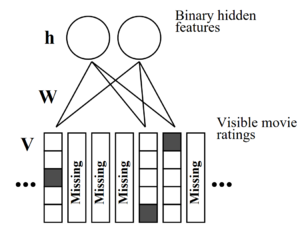
Salakhutdinov, Mnih, and Hinton framed the task of computing p(x_{im} = k | X?) as inference on an underlying RBM with trained parameters. The dataset is sub-divided into rating matrices, where a user’s ratings are one-hot encoded into a matrix V such that v?? = 1 if the user rates movie j with rating k. The figure above illustrates the RBM graph:

Salakhutdinov，Mnih和Hinton將計算p(x_ {im} = k |X?)的任務框架化為對具有訓練參數的基礎RBM的推斷。 數據集被細分為評分矩陣，其中用戶的評分被一次熱編碼到矩陣V中，如果用戶對影片j評分為k，則v??= 1。 上圖說明了RBM圖：

• V is a 5 x d matrix that corresponds to one-hot encoded integer ratings of the user.
  V是一個5 xd矩陣，對應于用戶的一鍵編碼整數評級。
• h is a F x 1 vector of binary hidden variables, where F is the number of hidden variables.
  h是二進制隱藏變量的F x 1向量，其中F是隱藏變量的數量。
• W is a d x F x 5 tensor that encodes adjacency between ratings and hidden features. Its entry W?c? corresponds to the edge potential between rating k of the movie j and the hidden feature c.
  W是adx F x 5張量，可對等級和隱藏特征之間的鄰接進行編碼。 它的項W?c?對應于電影j的等級k與隱藏特征c之間的邊緣電勢。

The whole user-item interaction matrix is a collection of V(s), where each V corresponds to each user’s ratings. Because each user can have different missing values, each will have a unique RBM graph. In each RBM graph, the edges connect ratings and hidden features but do not appear between items of missing ratings. The paper treats W as a set of edge potentials that are tied across all such RBM graphs.

整個用戶-項目交互矩陣是V (s) 的集合 ，其中每個V對應于每個用戶的等級 。 由于每個用戶可能具有不同的缺失值，因此每個用戶都有唯一的RBM圖。 在每個RBM圖中，邊連接等級和隱藏特征，但不會出現在缺少等級的項目之間。 本文將W視為邊緣電位集，這些邊緣電位綁在所有此類RBM圖上。

In the training phase, RBM characterizes the relationship between the ratings and hidden features using conditional probabilities p(v?? = 1 | h) and p(h? = 1 | V):

在訓練階段，RBM使用條件概率p(v??= 1 | h)和p(h?= 1 | V)來表征等級與隱藏特征之間的關系：

After getting these probabilities, there are two extra steps to compute p(v?? = 1 | V):

得到這些概率后，還有兩個額外的步驟來計算p(v??= 1 | V) ：

1. Compute the distribution of each hidden feature in h based on observed ratings V and the edge potentials W (p(h? = 1 | V) for each a).
   根據觀察到的等級V和邊緣電勢W(每個a的p(h?= 1 | V))計算h中每個隱藏特征的分布。
2. Compute p(v?? = 1 | V) based on the edge potentials W and the distribution of p(h? = 1 | V).
   根據邊緣電位W和p(h?= 1 | V)的分布計算p(v??= 1 | V)。

In the optimization phase, W is optimized by the marginal likelihood of V — p(V). The gradient ? W??? is computed using contrastive divergence, which is an approximation of the gradient-based on Gibbs sampling:

在優化階段，通過V_p (V)的邊際似然來優化W。 使用對比散度計算梯度?W，它是基于Gibbs采樣的基于梯度的近似值：

The expectation <.>_T represents a distribution of samples from running the Gibbs sampler, initialized at the data, for T full steps. T is typically set to 1 at the beginning of learning and increased as the learning converges. When running the Gibbs sampler, the RBM reconstructs (as seen in equation 1) the distribution over the non-missing ratings. The approximate gradients of contrastive divergence can then be averaged over all n users.

期望值<_> _ T代表運行Gibbs采樣器的采樣分布，并在數據上初始化了T個完整步驟。 T通常在學習開始時設置為1，并隨著學習收斂而增加。 運行吉布斯采樣器時，RBM會重建(如式1所示)非缺失等級上的分布。 然后可以在所有n個用戶上平均對比散度的近似梯度。

The PyTorch code of the RBM model class is given below for illustration purpose:

出于說明目的，以下給出了RBM模型類的PyTorch代碼：

class RBM:def __init__(self, n_vis, n_hid):"""Initialize the parameters (weights and biases) we optimize during the training process:param n_vis: number of visible units:param n_hid: number of hidden units"""# Weights used for the probability of the visible units given the hidden unitsself.W = torch.randn(n_hid, n_vis)  # torch.rand: random normal distribution mean = 0, variance = 1# Bias probability of the visible units is activated, given the value of the hidden units (p_v_given_h)self.v_bias = torch.randn(1, n_vis)  # fake dimension for the batch = 1# Bias probability of the hidden units is activated, given the value of the visible units (p_h_given_v)self.h_bias = torch.randn(1, n_hid)  # fake dimension for the batch = 1def sample_h(self, x):"""Sample the hidden units:param x: the dataset"""# Probability h is activated given that the value v is sigmoid(Wx + a)# torch.mm make the product of 2 tensors# W.t() take the transpose because W is used for the p_v_given_hwx = torch.mm(x, self.W.t())# Expand the mini-batchactivation = wx + self.h_bias.expand_as(wx)# Calculate the probability p_h_given_vp_h_given_v = torch.sigmoid(activation)# Construct a Bernoulli RBM to predict whether an user loves the movie or not (0 or 1)# This corresponds to whether the n_hid is activated or not activatedreturn p_h_given_v, torch.bernoulli(p_h_given_v)def sample_v(self, y):"""Sample the visible units:param y: the dataset"""# Probability v is activated given that the value h is sigmoid(Wx + a)wy = torch.mm(y, self.W)# Expand the mini-batchactivation = wy + self.v_bias.expand_as(wy)# Calculate the probability p_v_given_hp_v_given_h = torch.sigmoid(activation)# Construct a Bernoulli RBM to predict whether an user loves the movie or not (0 or 1)# This corresponds to whether the n_vis is activated or not activatedreturn p_v_given_h, torch.bernoulli(p_v_given_h)def train(self, v0, vk, ph0, phk):"""Perform contrastive divergence algorithm to optimize the weights that minimize the energyThis maximizes the log-likelihood of the model"""# Approximate the gradients with the CD algorithmself.W += (torch.mm(v0.t(), ph0) - torch.mm(vk.t(), phk)).t()# Add (difference, 0) for the tensor of 2 dimensionsself.v_bias = torch.sum((v0 - vk), 0)self.h_bias = torch.sum((ph0 - phk), 0)

For my PyTorch implementation, I designed the RBM architecture with a hidden layer of 100 units activated by a non-linear sigmoid function. Other hyper-parameters include the batch size of 512 and epochs of 50.

對于我的PyTorch實施 ，我設計了RBM架構，其中包含一個由非線性S型函數激活的100個單位的隱藏層。 其他超參數包括512的批量大小和50的時期。

2 —可解釋的受限Boltzmann機器，用于協同過濾 (2 — Explainable Restricted Boltzmann Machines for Collaborative Filtering)

Explanations for recommendations can have multiple benefits, including effectiveness (helping users to make the right decisions), efficiency (assisting users to make faster decisions), and transparency (revealing the reasoning behind the recommendations). In the case of RBM, which assigns a low-dimensional set of features to items in a latent space, it is difficult to interpret these learned features. Therefore, a massive challenge is to choose an interpretable technique with moderate prediction accuracy for RBM.

對建議的解釋可以帶來多種好處，包括有效性(幫助用戶做出正確的決定)，效率(幫助用戶做出更快的決定)和透明性(揭示建議背后的原因)。 對于RBM，它為潛在空間中的項目分配了一組低維特征，很難解釋這些學習到的特征。 因此， 一個巨大的挑戰是為RBM選擇一種具有中等預測精度的可解釋技術 。

Abdollahi and Nasraoui designed an RBM model for a collaborative filtering recommendation system that suggests items that are explainable while maintaining accuracy. The paper’s scope is limited to recommendations where no additional source of data is used in explanations, and where explanations for recommended items can be generated from the ratings given to these items, by the active user’s neighbors only.

Abdollahi和Nasraoui設計了一種用于協作過濾推薦系統的RBM模型，該模型建議了在保持準確性的同時可以解釋的項目。 本文的范圍僅限于建議，在這些建議中，無需在解釋中使用其他數據源，并且只能由活動用戶的鄰居根據對這些項目的評級生成推薦項目的解釋。

The main idea is that if many neighbors have rated the recommended item, then this could provide a basis upon which to explain the recommendations, using neighborhood-style explanation mechanisms. For user-based neighbor-style explanations, such as the one shown in the figure above, the Explainability Score of item i for user u is defined as:

主要思想是，如果許多鄰居對推薦項目進行了評分，則可以使用鄰域風格的解釋機制為解釋推薦提供依據。 對于基于用戶的鄰居風格的解釋，例如上圖所示，用戶i的項i的可解釋性分數定義為：

Here N_k (u) is the set of user u’s k neighbors, r_{x, i} is the rating of x on item i, and R_max is the maximum rating value of N_k (u) on i. Cosine similarity defines the neighborhood. Without loss of information, r_{x, i} is 0 for missing ratings, indicating that user x does not contribute to the user-based neighbor-style explanation of item i for user u. Therefore, the Explainability Score is between 0 and 1. Item i is explainable for user u only if its explainability score is larger than 0. When no explanation can be made, the explainability ratio would be 0.

這里N_k(u)是用戶u的k個鄰居的集合， r_ {x，i}是項i上x的等級， R_max是i上N_k(u)的最大等級。 余弦相似度定義了鄰域 。 在不丟失信息的情況下，r_ {x，i}對于缺失的評分為0，指示用戶x對用戶u的項i的基于用戶的鄰居樣式解釋沒有貢獻。 因此， 解釋性分數在0到1之間 。 僅當項目i的可解釋性得分大于0時，項目i才能為用戶u解釋。如果無法解釋，則可解釋性比率將為0。

The TensorFlow code of the RBM model class is given below for illustration purpose:

出于說明目的，以下給出了RBM模型類的TensorFlow代碼：

def rbm(movies_df):"""Implement RBM architecture in TensorFlow:param movies_df: data frame that stores movies information:return: variables to be used during TensorFlow training"""hiddenUnits = 100  # Number of hidden layersvisibleUnits = len(movies_df)  # Number of visible layers# Create respective placeholder variables for storing visible and hidden layer biases and weightsvb = tf.placeholder("float", [visibleUnits])  # Number of unique movieshb = tf.placeholder("float", [hiddenUnits])  # Number of featuresW = tf.placeholder("float", [visibleUnits, hiddenUnits])  # Weights that connect the hidden and visible layers# Pre-process the input datav0 = tf.placeholder("float", [None, visibleUnits])_h0 = tf.nn.sigmoid(tf.matmul(v0, W) + hb)h0 = tf.nn.relu(tf.sign(_h0 - tf.random_uniform(tf.shape(_h0))))# Reconstruct the pre-processed input data (Sigmoid and ReLU activation functions are used)_v1 = tf.nn.sigmoid(tf.matmul(h0, tf.transpose(W)) + vb)v1 = tf.nn.relu(tf.sign(_v1 - tf.random_uniform(tf.shape(_v1))))h1 = tf.nn.sigmoid(tf.matmul(v1, W) + hb)# Set RBM training parametersalpha = 0.1  # Set learning ratew_pos_grad = tf.matmul(tf.transpose(v0), h0)  # Set positive gradientsw_neg_grad = tf.matmul(tf.transpose(v1), h1)  # Set negative gradients# Calculate contrastive divergence to maximizeCD = (w_pos_grad - w_neg_grad) / tf.to_float(tf.shape(v0)[0])# Create methods to update the weights and biasesupdate_w = W + alpha * CDupdate_vb = vb + alpha * tf.reduce_mean(v0 - v1, 0)update_hb = hb + alpha * tf.reduce_mean(h0 - h1, 0)# Set error function (RMSE)err = v0 - v1err_sum = tf.sqrt(tf.reduce_mean(err * err))# Initialize variablescur_w = np.zeros([visibleUnits, hiddenUnits], np.float32)  # Current weightcur_vb = np.zeros([visibleUnits], np.float32)  # Current visible unit biasescur_hb = np.zeros([hiddenUnits], np.float32)  # Current hidden unit biasesprv_w = np.zeros([visibleUnits, hiddenUnits], np.float32)  # Previous weightprv_vb = np.zeros([visibleUnits], np.float32)  # Previous visible unit biasesprv_hb = np.zeros([hiddenUnits], np.float32)  # Previous hidden unit biasesreturn v0, W, vb, hb, update_w, prv_w, prv_vb, prv_hb, update_vb, update_hb, cur_w, cur_vb, cur_hb, err_sum

For my TensorFlow implementation, I designed the RBM architecture with a hidden layer of 100 units activated by a non-linear sigmoid function. Other hyper-parameters include the batch size of 512 and epochs of 50. I also showed a sample recommendation list for a hypothetical user with explainability scores included.

對于我的TensorFlow實現 ，我設計了RBM架構，其中包含一個由非線性S型函數激活的100個單位的隱藏層。 其他超參數包括512的批量大小和50的時期。我還顯示了一個假設用戶的示例推薦列表，其中包括可解釋性評分。

3 —用于協同過濾的神經自回歸分布估計器 (3 — Neural Autoregressive Distribution Estimator for Collaborative Filtering)

One of the issues with the RBM model is such that it suffers from inaccuracy and impractically long training time since: (1) training is intractable, and (2) variational approximation or Markov Chain Monte-Carlo is required. Uria, Cote, Gregor, Murray, and Larochelle proposed the so-called Neural Autoregressive Distribution Estimator (NADE), which is a tractable distribution estimator for high-dimensional binary vectors. The estimator computes the conditional probabilities of each element, given the other elements to its left in the binary vector, where all conditionals share the same parameters. The probability of the binary vector can then be obtained by taking the product of these conditionals. NADE can be optimized efficiently via back-propagation, instead of expensive inference required to handle latent variables as in the case of RBM.

RBM模型的問題之一是，由于以下原因，它存在著不精確和不切實際的長訓練時間的問題，因為：(1)訓練是棘手的，并且(2)需要變分近似或馬爾可夫鏈蒙特卡洛。 Uria，Cote，Gregor，Murray和Larochelle提出了所謂的神經自回歸分布估計器 (NADE)，它是高維二元向量的易處理的分布估計器。 給定其他元素在二進制向量中的左??側，其中所有條件共享相同的參數，估計器將計算每個元素的條件概率。 然后可以通過取這些條件的乘積來獲得二元向量的概率。 NADE可以通過反向傳播進行有效優化，而不是像RBM那樣處理潛在變量需要昂貴的推斷。

As shown in the NADE diagram below:

如下圖的NADE圖所示：

• In the input layer, units with value 0 are shown in black, while units with value 1 are shown in white. The dashed border represents a layer pre-activation.
  在輸入層中，值為0的單位以黑色顯示，而值為1的單位以白色顯示。 虛線邊框表示層預激活。
• The outputs x^_0 give predictive probabilities for each dimension of a vector x_0, given elements earlier in some order.
  輸出x ^ _0給定向量x_0的每個維度的預測概率，這些元素按某種順序更早地給出。
• There is no path of connections between an output and the value being predicted, or elements of x_0 later in the ordering.
  在輸出和要預測的值之間，或者在以后的順序中x_0的元素之間，沒有連接路徑。
• Arrows connected correspond to connections with shared parameters.
  連接的箭頭對應于具有共享參數的連接。

Zheng, Tang, Ding, and Zhou proposed CF-NADE, which is inspired by RBM-CF and NADE models, that models the distribution of user ratings. Suppose we have four movies: m1 (rating is 5), m2 (rating is 3), m3 (rating is 4), and m4 (rating is 2). More specifically, the procedure goes as follows:

Zheng，Tang，Ding和Zhou提出了CF-NADE ，該模型受RBM-CF和NADE模型的啟發，該模型對用戶評分的分布進行了建模。 假設我們有四部電影：m1(等級為5)，m2(等級為3)，m3(等級為4)和m4(等級為2)。 更具體地說，過程如下：

1. The probability that the user gives m1 5-star conditioned on nothing.
   用戶給予m1 5星的概率不受任何限制。
2. The probability that the user gives m2 3-star conditioned on giving m1 5-star.
   用戶給m2 3星的概率取決于給m1 5星的概率。
3. The probability that the user gives m3 4-star conditioned on giving m1 5-star and m2 3-star.
   用戶給出m3 4星的概率取決于給出m1 5星和m2 3星的條件。
4. The probability that the user gives m4 2-star conditioned on giving m1 5-star, m2 3-star, and m3 4-star.
   用戶給出m4 2星的概率以給出m1 5星，m2 3星和m3 4星為條件。

Mathematically speaking, CF-NADE models the joint probability of the rating vector r by the chain rule as:

從數學上講，CF-NADE通過鏈規則將評級向量r的聯合概率建模為：

• D is the number of items that the user has rated.
  D是用戶已評分的項目數。
• o is the D-tuple in the permutations of (1, 2, …, D).
  o是(1、2，...，D)排列中的D元組。
• m? ∈ {1, 2, …, M} is the index of the i-th rated item.
  m?∈{1,2，…，M}是第i個被評估項的索引。
• r? = (r?_{m_{o?}}, r?_{m_{o?}}, …, r?_{m_{oD}}) denotes the training case for user u.
  r?=(r?_{m_ {o?}}，r?_{m_ {o2}}，…，r?_{m_ {oD}})表示用戶u的訓練案例。
• r?_{m_{o?}} ∈ {1, 2, …, K} denotes the rating that the user gave to item m_{o?}.
  r?_{m_ {o?}}∈{1，2，…，K}表示用戶對項目m_ {o?}的評分。
• r?_{m_{o<?}} denotes the first i — 1 elements of r indexed by o.
  r?_{m_ {o <?}}表示由o索引的r的前i個元素。

To expand on the process of getting the conditionals in equation 5, CF-NADE first computes the hidden representation of dimension H given r?_{m_{o<?}} as follows:

為了擴展在等式5中獲得條件的過程，CF-NADE首先根據給定r?_{m_ {o <?}}來計算維H的隱藏表示，如下所示：

• g is the activation function.
  g是激活功能。
• W? is the connection matrix associated with rating k.
  W?是與等級k相關的連接矩陣。
• W?_{:,j} is the j-th column of W? and W?_{i,j} is an interaction parameter between the i-th hidden unit and item j with rating k.
  W?_ {:, j}是W?的第j列，W?_{i，j}是第i個隱藏單元與等級k的項目j之間的交互參數。
• c is the bias term.
  c是偏差項。

Using this hidden representation from equation 6, CF-NADE then computes s?_{m_{o?}} (r_{m_{o_{<i}}}), which is the score indicating the preference that the user gave rating k for item m_{o?}, given the previous ratings r_{m_{o_{<i}}}:

CF-NADE使用公式6中的隱藏表示，然后計算s?_{m_ {o?}}(r_ {m_ {o _ {<i}}})，該分數表示用戶對商品m_的評分為k的偏好。 {o?}，鑒于先前的評分r_ {m_ {o _ {<i}}}：

V? and b? are the connection matrix and the bias term associated with rating k, respectively, where k is bigger than or equal to j. Using this score from equation 7, the conditionals in equation 5 could be modeled as:

V?和b?分別是與矩陣k相關的連接矩陣和偏置項，其中k大于或等于j。 使用公式7中的分數，公式5中的條件可以建模為：

CF-NADE is optimized via minimization of the negative log-likelihood of p(r) in equation 5:

通過最小化公式5中p(r)的負對數似然來優化CF-NADE：

Ideally, the order of movies (represented by notation o) should follow the timestamps of ratings. However, the paper shows that random drawing can yield good performance.

理想情況下，電影的順序(用符號o表示)應遵循收視率的時間戳。 但是，本文表明，隨機繪制可以產生良好的性能。

The Keras code of the CF-NADE model class is given below for illustration purpose:

出于說明目的，下面給出了CF-NADE模型類的Keras代碼：

class NADE(Layer):def __init__(self, hidden_dim, activation, W_regularizer=None, V_regularizer=None,b_regularizer=None, c_regularizer=None, bias=False, args=None, **kwargs):self.init = initializers.get('uniform')self.bias = biasself.activation = activationself.hidden_dim = hidden_dimself.W_regularizer = regularizers.get(W_regularizer)self.V_regularizer = regularizers.get(V_regularizer)self.b_regularizer = regularizers.get(b_regularizer)self.c_regularizer = regularizers.get(c_regularizer)self.args = argssuper(NADE, self).__init__(**kwargs)def build(self, input_shape):"""Build the NADE architecture:param input_shape: Shape of the input"""self.input_dim1 = input_shape[1]self.input_dim2 = input_shape[2]self.W = self.add_weight(shape=(self.input_dim1, self.input_dim2, self.hidden_dim),initializer=self.init, name='{}_W'.format(self.name), regularizer=self.W_regularizer)if self.bias:self.c = self.add_weight(shape=(self.hidden_dim,), initializer=self.init,name='{}_c'.format(self.name), regularizer=self.c_regularizer)if self.bias:self.b = self.add_weight(shape=(self.input_dim1, self.input_dim2), initializer=self.init,name='{}_b'.format(self.name), regularizer=self.b_regularizer)self.V = self.add_weight(shape=(self.hidden_dim, self.input_dim1, self.input_dim2),initializer=self.init, name='{}_V'.format(self.name), regularizer=self.V_regularizer)super(NADE, self).build(input_shape)

For my Keras implementation, I designed NADE architecture with a hidden layer of 100 units optimized via Adam with a learning rate of 0.001. Other hyper-parameters include the batch size of 512 and epochs of 50.

對于我的 Keras 實施 ，我設計了NADE架構，該架構的隱藏層為100個單元，通過Adam進行了優化，學習率為0.001。 其他超參數包括512的批量大小和50的時期。

模型評估 (Model Evaluation)

You can check out all three Boltzmann Machines-based recommendation models that I built at this repository: https://github.com/khanhnamle1994/transfer-rec/tree/master/Boltzmann-Machines-Experiments.

您可以查看我在此存儲庫中建立的所有三個基于Boltzmann Machines的推薦模型： https : //github.com/khanhnamle1994/transfer-rec/tree/master/Boltzmann-Machines-Experiments 。

• The dataset is MovieLens 1M, similar to the three previous experiments that I have done using Matrix Factorization, Multilayer Perceptron, and Autoencoders. The goal is to predict the ratings that a user will give to a movie, in which the ratings are between 1 to 5.

  數據集是MovieLens 1M ，類似于我之前使用矩陣分解 ， 多層感知器和自動編碼 器進行的三個實驗。 目的是預測用戶對電影的評分，其中評分介于1到5之間。

• The evaluation metric is Root Mean Squared Error (RMSE) in this setting. In other words, I want to minimize the delta between the predicted rating and the actual rating.

  在此設置中，評估指標為均方根誤差(RMSE) 。 換句話說，我想最小化預測等級與實際等級之間的差異。

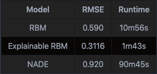
• The result table is at the bottom of my repo’s README: the explainable RBM model has the lowest RMSE and shortest training time, while the NADE model has the highest RMSE and longest training time.

  結果表在我的倉庫的README文件的底部：可解釋的RBM模型具有最低的RMSE和最短的訓練時間，而NADE模型具有最高的RMSE和最長的訓練時間。

結論 (Conclusion)

In this post, I have discussed the nuts and bolts of Boltzmann Machines and their use in collaborative filtering. I also walked through 3 different papers that use architectures inspired by Boltzmann Machines for the recommendation framework: (1) Restricted Boltzmann Machines, (2) Explainable Restricted Boltzmann Machines, and (3) Neural Autoregressive Distribution Estimator.

在本文中，我討論了Boltzmann機器的基本原理及其在協同過濾中的使用。 我還瀏覽了三篇不同的論文，這些論文使用了受Boltzmann機器啟發的體系結構作為推薦框架：(1)受限Boltzmann機器，(2)可解釋的受限Boltzmann機器和(3)神經自回歸分布估計器。

There are a couple of other papers worth being mentioned that I haven’t had time to go into details:

還有一些值得一提的論文，我還沒有時間詳細介紹：

• Georgiev and Nakov used RBMs to jointly model both: (1) the correlations between a user’s voted items and (2) the correlation between the users who voted a particular item to improve the accuracy of the recommendation system.

  Georgiev和Nakov使用RBM共同建模：(1)用戶投票項目之間的相關性；(2)對特定項目進行投票的用戶之間的相關性，以提高推薦系統的準確性。

• Hu et al. used RBM in group-based recommendation systems to model group preferences by jointly modeling collective features and group profiles.

  Hu等。 在基于組的推薦系統中使用RBM通過共同建模集體特征和組配置文件來對組偏好進行建模。

• Truyen et al. used Boltzmann machines to extract both: (1) the relation between a rated item and its rating (thanks to the connections between the hidden layer and the softmax layer) and (2) the correlations between rated items (thanks to the connections between the softmax layer units).

  Truyen等。 使用Boltzmann機器提取以下兩者：(1)額定項目與其額定值之間的關系(由于隱藏層和softmax層之間的連接)和(2)額定項目之間的相關性(由于softmax之間的連接圖層單位)。

• Gunawardana and Meek used Boltzmann machines not only for modeling correlation between users and items but also for integrating content information. More specifically, the model parameters are tied with the content information.

  Gunawardana和Meek不僅使用Boltzmann機器對用戶和物品之間的關聯進行建模，而且還用于集成內容信息。 更具體地說，模型參數與內容信息相關聯。

Stay tuned for the next blog post of this series that explores the various types of evaluation metrics in the context of recommendation systems.

請繼續關注本系列的下一篇博客文章，該文章在推薦系統的背景下探索各種類型的評估指標。

If you would like to follow my work on Recommendation Systems, Deep Learning, and Data Science Journalism, you can check out my Medium and GitHub, as well as other projects at https://jameskle.com/. You can also tweet at me on Twitter, email me directly, or find me on LinkedIn. Sign up for my newsletter to receive my latest thoughts on machine learning in research and production right at your inbox!

如果您想關注我在推薦系統，深度學習和數據科學新聞學方面的工作，可以 在 https://jameskle.com/ 上 查看我的 Medium 和 GitHub 以及其他項目 。 您也可以在Twitter在我的 微博 ， 直接給我發電子郵件 ，或者 找到我的LinkedIn 。 注冊我的時事通訊， 以在您的收件箱中接收我對研究和生產中的機器學習的最新想法！