與AI交易 (Trading with AI)

Stock markets tend to react very quickly to a variety of factors such as news, earnings reports, etc. While it may be prudent to develop trading strategies based on fundamental data, the rapid changes in the stock market are incredibly hard to predict and may not conform to the goals of more short term traders. This study aims to use data science as a means to both identify high potential stocks, as well as attempt to forecast future prices/price movement in an attempt to maximize an investor’s chances of success.

股票市場往往會對各種因素(例如新聞，收益報告等)??做出快速React。盡管基于基本數據制定交易策略可能是謹慎的做法，但股票市場的快速變化卻難以預測，而且可能無法預測符合更多短期交易者的目標。 這項研究旨在利用數據科學來識別高潛力股票，并試圖預測未來價格/價格走勢，以最大程度地提高投資者的成功機會。

In the first half of this analysis, I will introduce a strategy to search for stocks that involves identifying the highest-ranked stocks based on trading volume during the trading day. I will also include information based on twitter and sentiment analysis in order to provide an idea of which stocks have the maximum probability of going up in the near future. The next half of the project will attempt to apply forecasting techniques to our chosen stock(s). I will apply deep learning via a Long short term memory (LSTM) neural network, which is a form of a recurrent neural network (RNN) to predict close prices. Finally, I will also demonstrate how simple linear regression could aid in forecasting.

在本分析的前半部分，我將介紹一種搜索股票的策略，該策略涉及根據交易日內的交易量來確定排名最高的股票。 我還將包括基于推特和情緒分析的信息，以提供有關哪些股票在不久的將來具有最大上漲可能性的想法。 該項目的下半部分將嘗試將預測技術應用于我們選擇的股票。 我將通過長期短期記憶(LSTM)神經網絡應用深度學習，這是遞歸神經網絡(RNN)的一種形式，可以預測收盤價。 最后，我還將演示簡單的線性回歸如何有助于預測。

第1部分：庫存篩選 (Part 1: Stock screening)

Let’s begin by web-scraping data on the most active stocks in a given time period, in this case, one day. Higher trading volume is more likely to result in bigger price volatility which could potentially result in larger gains. The main python packages to help us with this task are the yahoo_fin, alpha_vantage, and pandas libraries.

首先，在給定的時間段(本例中為一天)中，通過網絡收集最活躍的股票的數據。 更高的交易量更有可能導致更大的價格波動，從而有可能帶來更大的收益。 可以幫助我們完成此任務的主要python軟件包是yahoo_fin ， alpha_vantage和pandas庫。

# Import relevant packages
import yahoo_fin.stock_info as ya
from alpha_vantage.timeseries import TimeSeries
from alpha_vantage.techindicators import TechIndicators
from alpha_vantage.sectorperformance import SectorPerformances
import pandas as pd
import pandas_datareader as web
import matplotlib.pyplot as plt
from bs4 import BeautifulSoup
import requests 
import numpy as np# Get the 100 most traded stocks for the trading day
movers = ya.get_day_most_active()
movers.head()

The yahoo_fin package is able to provide the top 100 stocks with the largest trading volume. We are interested in stocks with a positive change in price so let’s filter based on that.

yahoo_fin軟件包 能夠提供交易量最大的前100只股票。 我們對價格有正變化的股票感興趣，因此讓我們基于此進行過濾。

movers = movers[movers['% Change'] >= 0]
movers.head()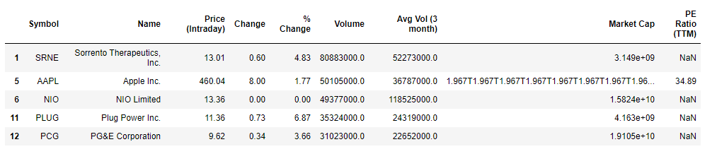

Excellent! We have successfully scraped the data using the yahoo_fin python module. it is often a good idea to see if those stocks are also generating attention, and what kind of attention it is to avoid getting into false rallies. We will scrap some sentiment data courtesy of sentdex. Sometimes sentiments may lag due to source e.g News article published an hour after the event, so we will also utilize tradefollowers for their twitter sentiment data. We will process both lists independently and combine them. For both the sentdex and tradefollowers data we use a 30 day time period. Using a single day might be great for day trading but increases the probability of jumping on false rallies. NOTE: Sentdex only has stocks that belong to the S&P 500. Using the BeautifulSoup library, this process is made fairly simple.

優秀的！ 我們已經使用yahoo_fin python模塊成功地抓取了數據。 通常，最好查看這些股票是否也引起關注，以及避免引起虛假集會的關注是什么。 我們將根據senddex刪除一些情感數據。 有時，情緒可能會由于消息來源而有所滯后，例如在事件發生后一小時發布的新聞文章，因此我們還將利用貿易關注者的推特情緒數據。 我們將獨立處理兩個列表并將其合并。 對于senddex和tradefollowers數據，我們使用30天的時間段。 使用單日交易對日間交易而言可能很棒，但會增加跳空虛假反彈的可能性。 注意：Sentdex僅擁有屬于S＆P 500的股票。使用BeautifulSoup庫，此過程變得相當簡單。

res = requests.get('http://www.sentdex.com/financial-analysis/?tf=30d')
soup = BeautifulSoup(res.text)
table = soup.find_all('tr')# Initialize empty lists to store stock symbol, sentiment and mentionsstock = []
sentiment = []
mentions = []
sentiment_trend = []# Use try and except blocks to mitigate missing data
for ticker in table:
    ticker_info = ticker.find_all('td')
    
    try:
        stock.append(ticker_info[0].get_text())
    except:
        stock.append(None)
    try:
        sentiment.append(ticker_info[3].get_text())
    except:
        sentiment.append(None)
    try:
        mentions.append(ticker_info[2].get_text())
    except:
        mentions.append(None)
    try:
        if (ticker_info[4].find('span',{"class":"glyphicon  glyphicon-chevron-up"})):
            sentiment_trend.append('up')
        else:
            sentiment_trend.append('down')
    except:
        sentiment_trend.append(None)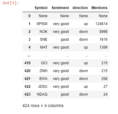

We then combine these results with our previous results about the most traded stocks with positive price changes on a given day. This done using a left join of this data frame with the original movers data frame

然后，我們將這些結果與我們先前的有關交易最多的股票的先前結果相結合，并得出給定價格的正變化。 使用此數據框與原始移動者數據框的左連接完成此操作

top_stocks = movers.merge(company_info, on='Symbol', how='left')
top_stocks.drop(['Market Cap','PE Ratio (TTM)'], axis=1, inplace=True)
top_stocks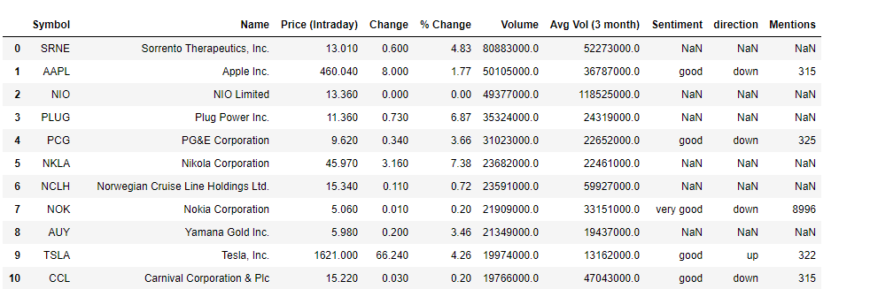

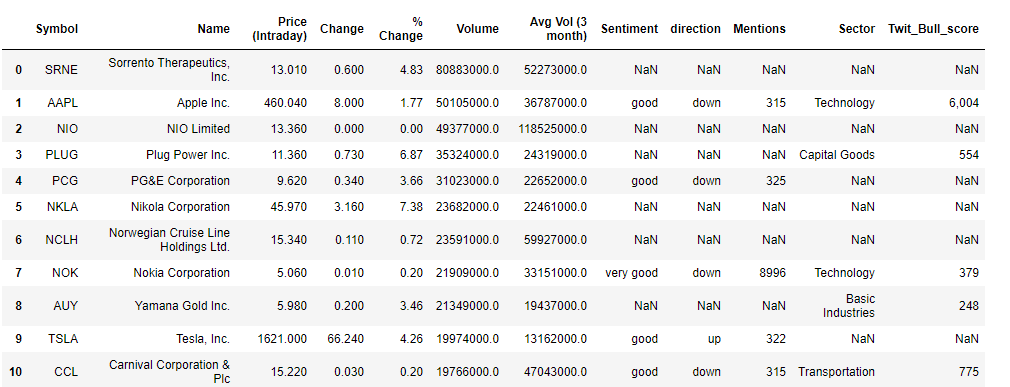
The movers data frame had a total of 45 stocks but for brevity only 10 are shown here. A couple of stocks pop up with both very good sentiments and an upwards trend in favourability. ZNGA, TWTR, and AES (not shown) for instance stood out as potentially good picks. Note, the mentions here refer to the number of times the stock was referenced according to the internal metrics used by sentdex. Let’s attempt supplementing this information with some data based on twitter. We get stocks that showed the strongest twitter sentiments within a time period of 1 month and were considered bullish.

推動者數據框中共有45種存量，但為簡潔起見，此處僅顯示10種。 情緒高漲且有利可圖的趨勢呈上升趨勢的幾只股票。 例如，ZNGA，TWTR和AES(未顯示)脫穎而出，成為潛在的好選擇。 請注意，此處提及的內容是指根據senddex使用的內部指標引用股票的次數 。 讓我們嘗試使用基于Twitter的一些數據來補充此信息。 我們得到的股票在1個月內顯示出最強烈的Twitter情緒，并被視為看漲。

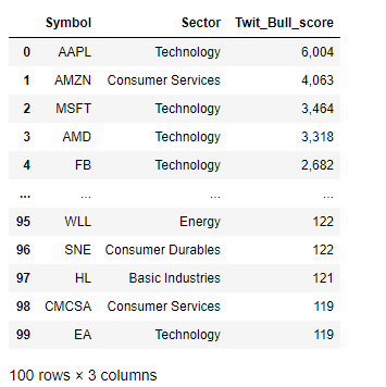
Twit_Bull_score refers to the internal scoring used at tradefollowers to rank stocks that are considered bullish, based on twitter sentiments, and can range from 1 to as high as 10,000 or greater. With the twitter sentiments obtained, I’ll combine it with our sentiment data to get an overall idea of the stocks and their sentiments

Twit_Bull_score指的是在所使用的內部計分tradefollowers到秩股被認為看漲，基于在twitter情緒，并且范圍可以從1至高達10,000或更大。 在獲得推特情緒后，我將其與情緒數據結合起來以全面了解股票及其情緒

For completeness, stocks classified as having large momentum and their sentiment data will also be included in this analysis. These were scraped and merged with the Final_list data frame.

為了完整起見，被歸類為動量較大的股票及其情緒數據也將包括在此分析中。 這些內容已被抓取并與Final_list數據框合并。

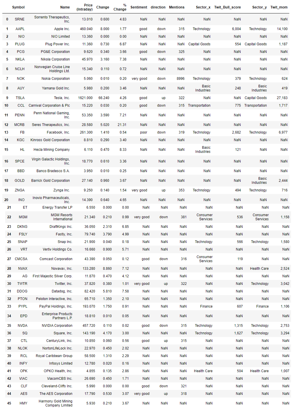
Our list now contains even more information to help us with our trades. Stocks that it suggests might generate positive returns include TSLA, ZNGA, and TWTR as their sentiments are positive, and they have relatively decent twitter sentiment scores. As an added measure, we can also obtain information on the sectors to see how they’ve performed. Again, we will use a one month time period for comparison. The aforementioned stocks belong to the Technology and consumer staples sectors.

我們的清單現在包含更多信息，以幫助我們進行交易。 它暗示可能產生正回報的股票包括TSLA，ZNGA和TWTR，因為它們的情緒是積極的，并且它們的Twitter情緒得分相對不錯。 作為一項附加措施，我們還可以獲得有關部門的信息，以了解其表現。 同樣，我們將使用一個月的時間進行比較。 上述股票屬于技術和消費必需品領域。

# Checking sector performancessp = SectorPerformances(key='0E66O7ZP6W7A1LC9', output_format='pandas')
plt.figure(figsize=(8,8))
data, meta_data = sp.get_sector()
print(meta_data)
data['Rank D: Month Performance'].plot(kind='bar')
plt.title('One Month Performance (%) per Sector')
plt.tight_layout()
plt.grid()
plt.show()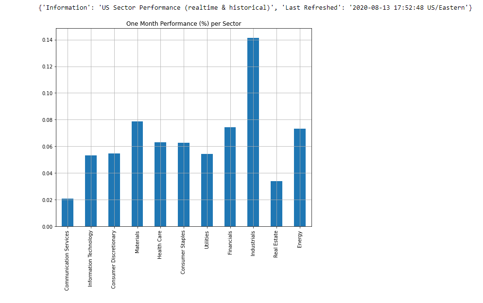

The industrials sector appears to be the best performing in this time period. Consumer staples sector appears to be doing better than the information technology sector, but overall they are up which bodes well for potential investors. Of course with stocks, a combination of news, technical and fundamental analysis, as well as knowledge of the given product/sector, is needed to effectively invest but this system is designed to find stocks that are more likely to perform.

在這段時間內，工業部門表現最好。 消費必需品領域似乎比信息技術領域做得更好，但總體而言，它們的增長對潛在的投資者來說是個好兆頭。 當然，對于庫存而言，需要新聞，技術和基本面分析以及對給定產品/行業的知識的組合才能有效地進行投資，但是此系統旨在查找更有可能執行的庫存。

To validate this notion, let’s construct a mock portfolio using TSLA, ZNGA, and TWTR as our chosen stocks and observe their cumulative returns. This particular analysis began on the 13th of August, 2020 so that will be the starting date of the investments.

為了驗證這一觀點，讓我們使用TSLA，ZNGA和TWTR作為我們選擇的股票來構建模擬投資組合，并觀察它們的累積收益。 這項特殊的分析始于2020年8月13日，因此這將是投資的開始日期。

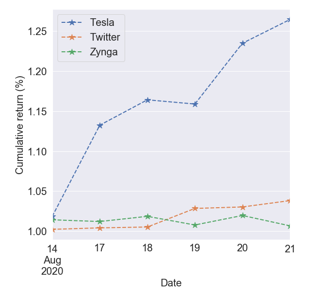
Overall all three investments would have netted a positive net return over the 7-day period. The tesla stock especially experienced a massive jump around the 14th and 19th respectively, while twitter shows a continued upward trend.

總體而言，所有這三筆投資在7天之內都將獲得正的凈回報。 特斯拉股票分別在14日和19日經歷了大幅上漲，而Twitter則顯示出持續上升的趨勢。

Please note that this analysis is only a guide to find potentially positive return generating stocks and does not guarantee positive returns. It is still up to the investor to do the research.

請注意，此分析只是尋找可能產生正回報的股票的指南，并不保證正回報。 仍由投資者來進行研究。

第2部分：使用LSTM預測收盤價 (Part 2: Forecasting close price using an LSTM)

In this section, I will attempt to apply deep learning to a stock of our choosing to forecast future prices. At the time this project was conceived (early mid-late July 2020), the AMD stock was selected as it experienced really high gains around this time. First I obtain stock data for our chosen stock. Data from 2014 data up till August of 2020 was obtained for our analysis. Our data will be obtained from yahoo using the pandas_webreader package

在本部分中，我將嘗試將深度學習應用于我們選擇的股票以預測未來價格。 在構想該項目時(2020年7月中下旬)，選擇AMD股票是因為它在這段時間獲得了非常高的收益。 首先，我獲取所選股票的股票數據。 我們從2014年數據到2020年8月的數據進行了分析。 我們的數據將使用pandas_webreader包從雅虎獲得。

# Downloading stock data using the pandas_datareader libraryfrom datetime import datetimestock_dt = web.DataReader('AMD','yahoo',start,end)
stock_dt.reset_index(inplace=True)
stock_dt.head()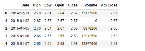

Next, some technical indicators were obtained for the data using the alpha_vantage python package.

接下來，使用alpha_vantage python軟件包為數據獲取了一些技術指標。

# How to obtain technical indicators for a stock of choice
# RSI
t_rsi = TechIndicators(key='0E66O7ZP6W7A1LC9',output_format='pandas')
data_rsi, meta_data_rsi = t_rsi.get_rsi(symbol='AMD', interval='daily',time_period = 9,
                          series_type='open')# Bollinger bands
t_bbands = TechIndicators(key='0E66O7ZP6W7A1LC9',output_format='pandas')
data_bbands, meta_data_bb = t_bbands.get_bbands(symbol='AMD', interval='daily', series_type='open', time_period=9)

This can easily be functionalized depending on the task. To learn more about technical indicators and how they are useful in stock analysis, I welcome you to explore investopedia’s articles on different technical indicators. Differential data was also included in the list of features for predicting stock prices. In this study, differential data refers to the difference between price information on 2 consecutive days (price at time t and price at time t-1).

可以根據任務輕松地對其進行功能化。 要了解有關技術指標的更多信息，以及它們如何在庫存分析中發揮作用 ，我歡迎您瀏覽investopedia關于不同技術指標的文章。 差異數據也包含在用于預測股價的功能列表中。 在這項研究中，差異數據是指連續2天的價格信息之間的差異(時間t的價格和時間t-1的價格)。

特征工程 (Feature engineering)

Let’s visualize how the generated features relate to each other using a heatmap of the correlation matrix.

讓我們使用相關矩陣的熱圖可視化生成的特征如何相互關聯。

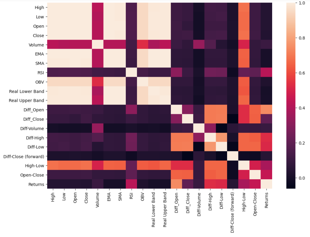
The closing price has very strong correlations with some of the other price information such as opening price, highs, and lows. On the other hand, the differential prices aren't as correlated. We want to limit the amount of colinearity in our system before running any machine learning routine. So feature selection is a must.

收盤價與其他一些價格信息(例如開盤價，最高價和最低價)具有非常強的相關性。 另一方面，差異價格卻不相關。 我們希望在運行任何機器學習例程之前限制系統中的共線性量。 因此，功能選擇是必須的。

I utilize two means of feature selection in this section. Random forests and mutual information gain. Random forests are very popular due to their relatively good accuracy, robustness as well as simplicity in terms of utilization. They can directly measure the impact of each feature on the accuracy of the model and in essence, give them a rank. Information gain, on the other hand, calculates the reduction in entropy from transforming a dataset in some way. Mutual information gain essentially evaluates the gain of each variable in the context of the target variable.

在本節中，我采用兩種功能選擇方式。 隨機森林和相互信息獲取。 隨機森林由于其相對較高的準確性，魯棒性和使用簡單性而非常受歡迎。 他們可以直接測量每個功能對模型準確性的影響，并從本質上給他們一個排名。 另一方面，信息增益通過某種方式轉換數據集來計算熵的減少。 互信息增益本質上是在目標變量的上下文中評估每個變量的增益。

隨機森林回歸 (Random forest regressor)

Let’s make a temporary training and testing data sets and run the regressor on it.

讓我們做一個臨時的訓練和測試數據集，并在其上運行回歸器。

# Feature selection using a Random forest regressor
X_train, X_test,y_train, y_test = train_test_split(X,y,test_size=0.2,random_state=0)feat = SelectFromModel(RandomForestRegressor(n_estimators=100,random_state=0,n_jobs=-1))
feat.fit(X_train,y_train)X_train.columns[feat.get_support()]

The regressor essentially selected the features that displayed a good correlation with the close price which is the target variable. However, although it selected the most important we would like information on the information gain from each variable. An issue with using random forests is it tends to diminish the importance of other correlated variables and may lead to incorrect interpretation. However, it does help reduce overfitting. Using the regressor, only three features were seen as being useful for prediction; High, Low, and Open prices.

回歸器實質上選擇了與作為目標變量的收盤價顯示出良好相關性的特征。 但是，盡管它選擇了最重要的信息，我們還是希望獲得有關每個變量的信息增益的信息。 使用隨機森林的一個問題是，它往往會降低其他相關變量的重要性，并可能導致錯誤的解釋。 但是，它確實有助于減少過度擬合。 使用回歸器，只有三個特征被認為對預測有用。 高，低和開盤價。

相互信息獲取 (Mutual information gain)

Now quantitatively see how each feature contributes to the prediction

現在定量了解每個特征如何有助于預測

from sklearn.feature_selection import mutual_info_regression, SelectKBestmi = mutual_info_regression(X_train,y_train)
mi = pd.Series(mi)
mi.index = X_train.columns
mi.sort_values(ascending=False,inplace=True)mi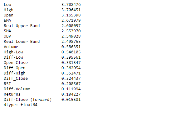

The results validate the results using the random forest regressor, but it appears some of the other variables also contribute a decent amount of information. In terms of selection, only features with contributions greater than 2 are selected, resulting in 8 features

結果使用隨機森林回歸器驗證了結果，但似乎其他一些變量也提供了可觀的信息量。 在選擇方面，僅會選擇貢獻大于2的特征，從而產生8個特征

LSTM的數據準備 (Data preparation for the LSTM)

In order to construct a Long short term memory neural network (LSTM), we need to understand its structure. Below is the design of a typical LSTM unit.

為了構建長期短期記憶神經網絡(LSTM)，我們需要了解其結構。 以下是典型LSTM單元的設計。

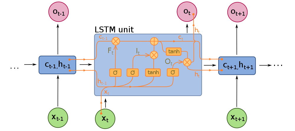
As mentioned earlier, LSTM’s are a special type of recurrent neural network (RNN). Recurrent neural networks (RNN) are a special type of neural network in which the output of a layer is fed back to the input layer multiple times in order to learn from the past data. Basically, the neural network is trying to learn data that follows a sequence. However, since the RNNs utilize past data, they can become computationally expensive due to storing large amounts of data in memory. The LSTM mitigates this issue, using gates. It has a cell state, and 3 gates; forget, input and output gates.

如前所述， LSTM是一種特殊的遞歸神經網絡( RNN )。 遞歸神經網絡( RNN )是一種特殊的神經網絡，其中層的輸出多次反饋到輸入層，以便從過去的數據中學習。 基本上，神經網絡正在嘗試學習遵循序列的數據。 但是，由于RNN利用過去的數據，由于在內存中存儲大量數據，它們可能會在計算上變得昂貴。 LSTM使用蓋茨緩解了此問題。 它具有單元狀態和3個門。 忘記 ， 輸入和輸出門。

The cell state is essentially the memory of the network. It carries information throughout the data sequence processing. Information is added or removed from this cell state using gates. Information from the previous hidden state and current input are combined and passed through a sigmoid function at the forget gate. The sigmoid function determines which data to keep or forget. The transformed values are then multiplied by the current cell state.

單元狀態本質上是網絡的內存。 它在整個數據序列處理過程中都承載信息。 使用門從該單元狀態添加或刪除信息。 來自先前隱藏狀態和當前輸入的信息將組合在一起，并通過遺忘門處的S型函數傳遞。 乙狀結腸功能決定要保留或忘記哪些數據。 然后將轉換后的值乘以當前單元格狀態 。

Next, the information from the previous hidden state (H_(t-1))combined with the input (X_t) is passed through a sigmoid function at the input gate to again determine important information, and also a tanh function to transform data between -1 and 1. This transformation helps with the stability of the network and helps deal with the vanishing/exploding gradient problem. These 2 outputs are multiplied together, and the output is added to the current cell state with the sigmoid function applied to it to give us our new cell state for the next time step.

接下來，來自先前隱藏狀態( H_(t-1) )的信息與輸入( X_t )的組合將通過輸入門的S型函數再次確定重要信息，以及通過tanh函數在-之間轉換數據1和1。此轉換有助于網絡的穩定性，并有助于解決消失/爆炸梯度問題。 將這兩個輸出相乘，然后將輸出加到當前單元格狀態，并應用sigmoid函數，為下一步提供新的單元格狀態。

Finally, the information from the hidden state combined with the current input is combined and a sigmoid function applied to it. In addition, the new cell state is passed through a tanh function to transform the values and both outputs are multiplied to determine the new hidden state for the next time step at the output gate.

最后，將來自隱藏狀態的信息與當前輸入組合在一起，并對其應用S型函數。 此外，新的小區狀態是通過雙曲正切函數傳遞給變換值和兩個輸出相乘以確定用于在輸出門在下一時間步驟將新的隱藏狀態。

Now we have an idea of how the LSTM works, let’s construct one. First, we split our data into training and test set. An 80 – 20 split was used for the training and test sets respectively in this case. The data were then scaled using a MinMaxScaler.

現在我們有了LSTM的工作原理，讓我們構造一個。 首先，我們將數據分為訓練和測試集。 在這種情況下，分別將80 – 20的比例用于訓練和測試集。 然后使用MinMaxScaler縮放數據。

LSTM的數據輸入結構 (Structure of data input for LSTM)

The figure below shows how the sequential data for an LSTM is constructed to be fed into the network. Data source: Althelaya et al, 2018

下圖顯示了如何構造LSTM的順序數據以饋入網絡。 數據來源： Althelaya等人，2018

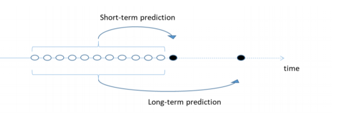
The idea is since stock data is sequential, information on a given day is related to information from previous days. Basically for data at time t, with a window size of N, the target feature will be the data point at time t, and the feature will be the data points [t-1, t-N]. We then sequentially move forward in time using this approach. This applies for the short-term prediction. For long term prediction, the target feature will be Fk time steps away from the end of the window where Fk is the number of days ahead we want to predict. We, therefore, need to format our data that way.

這個想法是因為庫存數據是連續的，所以給定日期的信息與前幾天的信息有關。 基本上對于時間t的數據，窗口大小為N ，目標特征將是時間t的數據點，特征將是數據點[ t-1 ， tN ]。 然后，我們使用此方法按時間順序向前移動。 這適用于短期預測。 對于長期預測，目標特征將是距窗口末端的Fk時間步長，其中Fk是我們要預測的提前天數。 因此，我們需要以這種方式格式化數據。

# Formatting input data for LSTM
def format_dataset(X, y, time_steps=1):
    Xs, ys = [], []
    for i in range(len(X) - time_steps):
        v = X.iloc[i:(i + time_steps)].values
        Xs.append(v)        
        ys.append(y.iloc[i + time_steps])
    return np.array(Xs), np.array(ys)

Following the work of Althelaya et al, 2018, a time window of 10 days was used for N.

繼Althelaya等人(2018年)的工作之后， N使用了10天的時間窗口。

建立LSTM模型 (Building the LSTM model)

The new installment of TensorFlow (Tensorflow 2.0) via Keras has made the implementation of deep learning models much easier than in previous installments. We will apply a bidirectional LSTM as they have been shown to more effective in certain applications (see Althelaya et al, 2018). This due to the fact that the network learns using both past and future data in 2 layers. Each layer performs the operations using reversed time steps to each other. The loss function, in this case, will be the mean squared error, and the adam optimizer with the default learning rate is applied. 20% of the training set will also be used as a validation set while running the model.

通過Keras的TensorFlow新版(Tensorflow 2.0)使深度學習模型的實現比以前的版本容易得多。 我們將應用雙向LSTM，因為它們已被證明在某些應用中更有效(請參見Althelaya等人，2018年 )。 這是由于網絡在2層中同時使用過去和將來的數據進行學習。 每一層使用彼此相反的時間步長執行操作。 在這種情況下，損失函數將是均方誤差，并且將使用具有默認學習率的adam優化器。 運行模型時，訓練集的20％也將用作驗證集。

# Design and input arguments into the LSTM model for stock price predictionfrom tensorflow import keras# Build model. Include 20% drop out to minimize overfitting
model = keras.Sequential()
model.add(keras.layers.Bidirectional(
        keras.layers.LSTM(
          units=32, 
          input_shape=(X_train_lstm.shape[1], X_train_lstm.shape[2]))
  )
)model.add(keras.layers.Dropout(rate=0.2))
model.add(keras.layers.Dense(units=1))# Define optimizer and metric for loss function
model.compile(optimizer='adam',loss='mean_squared_error')# Run model
history = model.fit(
    X_train_lstm, y_train_lstm, 
    epochs=90, 
    batch_size=40, 
    validation_split=0.2,
    shuffle=False,
    verbose=1   
)

Note we do not shuffle the data in this case. That’s because stock data is sequential i.e the price on a given day is dependent on the price from previous days. Now let’s have a look at the loss function to see how the validation and training data fair

請注意，在這種情況下，我們不會對數據進行混洗。 這是因為庫存數據是連續的，即給定日期的價格取決于前幾天的價格。 現在讓我們看一下損失函數，看看驗證和訓練數據如何公平

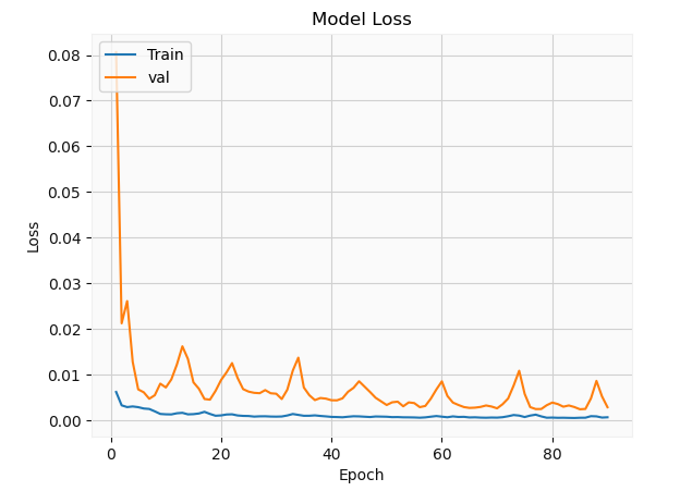
The validation set appears to have a lot more fluctuations relative to the training set. This is mainly due to the fact that most neural networks use stochastic gradient descent in minimizing the loss function which tends to be stochastic in nature. In addition, the data is batched which can influence the behavior of the solution. Of course, ideally, these hyper-parameters need to be optimized, but this is merely a simple demonstration. Let’s have a look at the solution

相對于訓練集，驗證集似乎有更多的波動。 這主要是由于以下事實：大多數神經網絡使用隨機梯度下降來使損失函數最小化，而損失函數在本質上往往是隨機的。 此外，數據會被批處理，這可能會影響解決方案的行為。 當然，理想情況下，需要優化這些超參數，但這僅僅是一個簡單的演示。 讓我們看一下解決方案

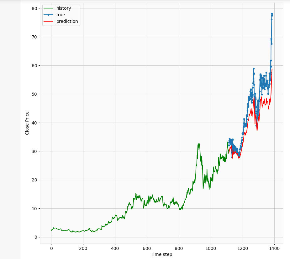
Overall, it seems the predictions follow the trend of the actual prices. Of course with more epochs and hyperparameter tuning, we could achieve better results. Let’s take a closer look

總體而言，似乎這些預測遵循實際價格的趨勢。 當然，通過更多的時期和超參數調整，我們可以獲得更好的結果。 讓我們仔細看看

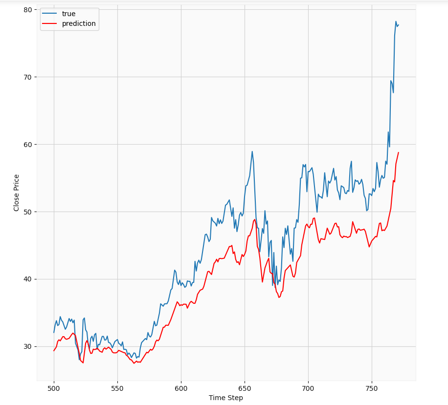
At first glance, we notice the LSTM has some implicit autocorrelation in its results since its predictions for a given day are very similar to those of the previous day. The predictions essentially lag the true results. Its basically showing that the best guess of the model is very similar to previous results. This should not be a surprising result; The stock market is influenced by a number of factors such as news, earnings reports, mergers, etc. Therefore, it is a bit too chaotic and stochastic to be accurately modeled because it depends on so many factors, some of which can be sporadic i.e positive or negative news. Therefore, in my opinion, this may not be the best way to predict stock prices. Of course with major advances in AI, there might actually be a way of doing this using LSTMs, but I don’t think the hedge funds will be sharing their methods with outsiders anytime soon.

乍一看，我們注意到LSTM在其結果中具有一些隱式自相關，因為它在給定日期的預測與前一天的預測非常相似。 這些預測實質上落后于真實結果。 它基本上表明，模型的最佳猜測與以前的結果非常相似。 這應該不足為奇； 股票市場受到許多因素的影響，例如新聞，收益報告，合并等。因此，它過于混亂和隨機，無法準確建模，因為它取決于太多因素，其中一些因素可能是零星的，即正面或負面新聞。 因此，我認為，這可能不是預測股價的最佳方法。 當然，隨著AI的重大進步，實際上可能有一種使用LSTM做到這一點的方法，但是我認為對沖基金不會很快與外界共享其方法。

第3部分：使用回歸分析估算價格走勢 (Part 3: Estimating price movement with regression analysis)

Of course, we could still make an attempt to have an idea of what the possible price movements might be. In this case, I will utilize the differential prices as there is less variance compared to using absolute prices. This is a somewhat naive way but let’s try it nevertheless. Let’s explore some relationships

當然，我們仍然可以嘗試了解價格可能發生的變化。 在這種情況下，我將利用差異價格，因為與使用絕對價格相比，差異較小。 這是一種比較幼稚的方法，但是還是請嘗試一下。 讓我們探索一些關系

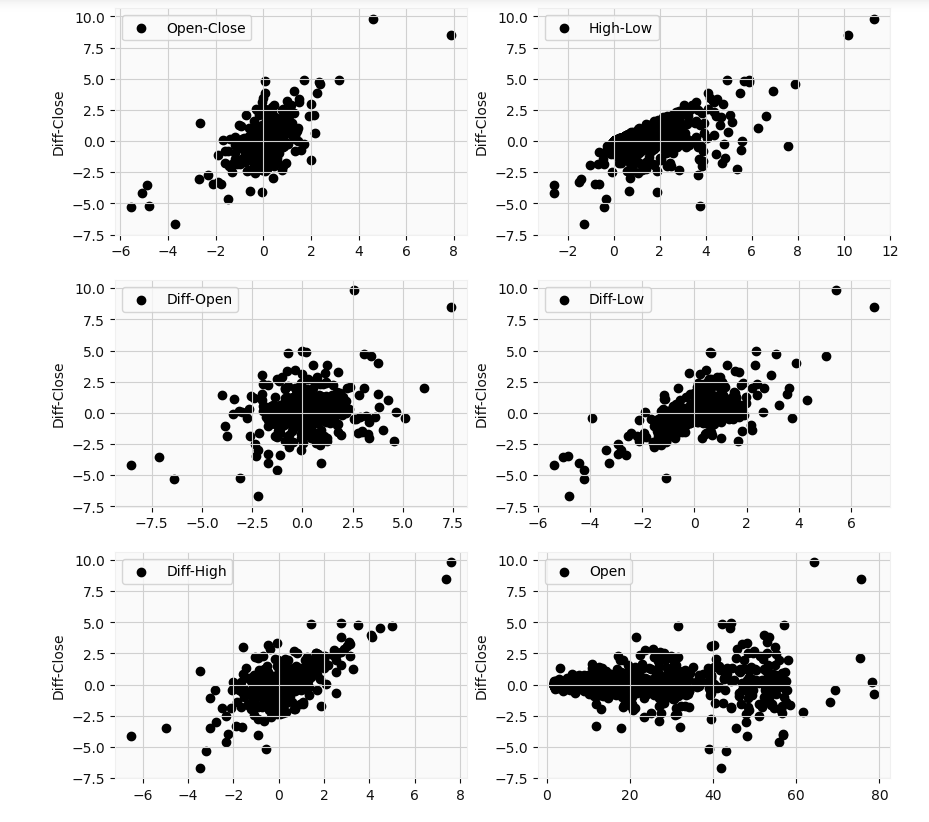
Again to reiterate, the differential prices relate to the difference between the price at time t and the previous day value at time t-1. The differential high, differential low, differential high-low, and differential open-close price appear to have a linear relationship with the differential close. But only the differential open-close would be useful in analysis. This because on a given day (time t), we can not know what the highs or lows are beforehand till the end of the trading day. Theoretically, those values could end up coinciding with the closing price. However, we do know the open value at the start of the trading period. I will apply ridge regression to make our results more robust. Our target variable will be the differential close price, and our feature will be the differential open-close price.

再次重申，差異價格與時間t的價格和時間t-1的前一天值之間的差有關。 差價高，差價低，差價高低和差價開盤價與差價收盤價似乎具有線性關系。 但是，只有微分開閉對分析有用。 這是因為在給定的一天(時間t )，我們直到交易日結束之前都不知道高點或低點是什么。 從理論上講，這些價值最終可能與收盤價一致。 但是，我們確實知道交易期開始時的未平倉價。 我將應用嶺回歸來使我們的結果更可靠。 我們的目標變量將是差異收盤價，而我們的特征將是差異開盤價。

from sklearn.linear_model import LinearRegression, Ridge, Lasso
from sklearn.model_selection import GridSearchCV, cross_val_score
import sklearn
from sklearn.metrics import median_absolute_error, mean_squared_error# Split data into training and test
X_train_reg, X_test_reg, y_train_reg, y_test_reg = train_test_split(X_reg, y_reg, test_size=0.2, random_state=0)# Use a 10-fold cross validation to determine optimal parameters for a ridge regression
ridge = Ridge()
alphas = [1e-15,1e-8,1e-6,1e-5,1e-4,1e-3,1e-2,1e-1,0,1,5,10,20,30,40,45,50,55,100]
params = {'alpha': alphas}ridge_regressor = GridSearchCV(ridge,params, scoring='neg_mean_squared_error',cv=10)
ridge_regressor.fit(X_reg,y_reg)print(ridge_regressor.best_score_)
print(ridge_regressor.best_params_)

The neg_mean_squared_error returns the negative version of the mean squared error. The closer it is to 0, the better the model. The cross-validation returned an alpha value of 1e-15 and a score of approximately -0.4979. Now let’s run the actual model and see our results

neg_mean_squared_error返回均方誤差的負版本。 距離0越近，模型越好。 交叉驗證返回的alpha值為1e-15，得分約為-0.4979。 現在讓我們運行實際模型并查看我們的結果

regr = Ridge(alpha=1e-15)
regr.fit(X_train_reg, y_train_reg)y_pred = regr.predict(X_test_reg)
y_pred_train = regr.predict(X_train_reg)print(f'R^2 value for test set is {regr.score(X_test_reg,y_test_reg)}')
print(f'Mean squared error is {mean_squared_error(y_test_reg,y_pred)}')plt.scatter(df_updated['Open-Close'][1:],df_updated['Diff_Close'][1:],c='k')
plt.plot(df_updated['Open-Close'][1:], (regr.coef_[0] * df_updated['Open-Close'][1:] + regr.intercept_), c='r' );
plt.xlabel('Open-Close')
plt.ylabel('Diff-Close')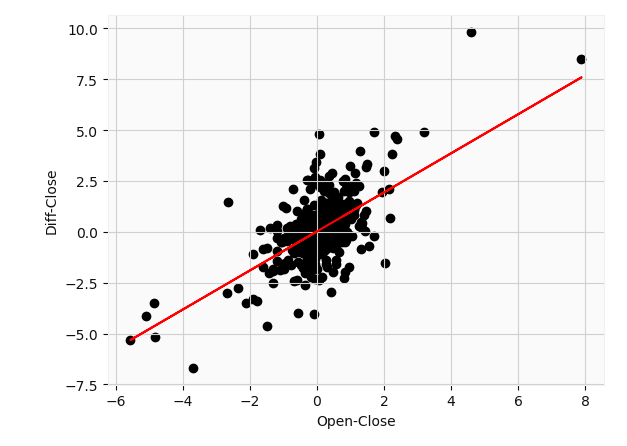

The model corresponds to a slope of $0.9599 and an intercept of $0.01854. This basically says that for every $1 increase in price between the opening price on a given day, and its previous closing price we can expect the closing price to increase by roughly a dollar from its closing price the day before. I obtained a mean square error of 0.58 which is fairly moderate all things considered. This R2 value of 0.54 basically says 54% of the variance in the differential close price is explained by the differential open-close price. Not so bad so far. Note that the adjusted R2 value was roughly equal to the original value.

該模型對應的斜率是0.9599美元 ，截距是0.01854美元。 這基本上就是說，在給定日期的開盤價與其之前的收盤價之間，每增加1美元的價格，我們就可以預期收盤價比前一天的收盤價增加大約1美元。 我獲得了0.58的均方誤差，考慮到所有因素，該誤差相當適中。 R2值為0.54基本上表示差異收盤價差異的54％由差異開盤價解釋。 到目前為止還算不錯。 請注意，調整后的R2值大致等于原始值。

To be truly effective, we need to make further use of statistics. Specifically, let’s define a prediction interval around the model. Prediction intervals give you a range for the prediction that accounts for any threshold of modeling error. Prediction intervals are most commonly used when making predictions or forecasts with a regression model, where a quantity is being predicted. We select the 99% confidence interval in this example such that our actual predictions fall into this range 99% of the time. For an in-depth overview and explanation please explore machinelearningmastery

為了真正有效，我們需要進一步利用統計數據。 具體來說，讓我們在模型周圍定義一個預測間隔。 預測間隔為您提供了一個預測范圍，該范圍考慮了建模誤差的任何閾值。 預測間隔是在預測數量的回歸模型中進行預測或預測時最常使用的時間間隔。 在此示例中，我們選擇99％置信區間，以使我們的實際預測有99％的時間處于該范圍內。 有關深入的概述和說明，請瀏覽機器學習知識。

def predict_range(X,y,model,conf=2.58):
    
    from numpy import sum as arraysum
    
    # Obtain predictions
    yhat = model.predict(X)
    
    # Compute standard deviation
    sum_errs = arraysum((y - yhat)**2)
    stdev = np.sqrt(1/(len(y)-2) * sum_errs)
   
    # Prediction interval (default confidence: 99%)
    interval = conf * stdev
    
    lower = []
    upper = []
    
    for i in yhat:
        lower.append(i-interval)
        upper.append(i+interval)return lower, upper, interval

Let’s see our prediction intervals

讓我們看看我們的預測間隔

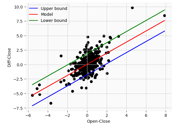
Our prediction error corresponds to a value of $1.82 in this example. Of course, the parameters used to obtain our regression model (slope and intercept) also have a confidence interval which we could calculate, but its the same process as highlighted above. From this plot, we can see that even with a 99% confidence interval, some values still fall outside the range. This highlights just how difficult it is to forecast stock price movements. So ideally we would supplement our analysis with news, technical indicators, and other parameters. In addition, our model is still quite limited. We can only make predictions about the closing price on the same day i.e at time t. Even with the large uncertainty, this could potentially prove useful in, for instance, options tradings.

在此示例中，我們的預測誤差對應于$ 1.82的值。 當然，用于獲得回歸模型的參數(斜率和截距)也具有我們可以計算的置信區間，但其過程與上面突出顯示的過程相同。 從該圖可以看出，即使置信區間為99％，某些值仍落在該范圍之外。 這突顯了預測股價走勢的難度。 因此，理想情況下，我們將使用新聞，技術指標和其他參數來補充我們的分析。 此外，我們的模型仍然非常有限。 我們只能對當天(即時間t)的收盤價做出預測。 即使存在很大的不確定性，這也可能在例如期權交易中被證明是有用的。

這是什么意思呢？ (What does this all mean?)

The stock screening strategy introduced could be a valuable tool for finding good stocks and minimizing loss. Certainly, in future projects, I could perform sentiment analysis myself in order to get information on every stock from the biggest movers list. There is also some room for improvement in the LSTM algorithm. If there was a way to minimize the bias and eliminate the implicit autocorrelation in the results, I’d love to hear about it. So far, the majority of research on the topic haven’t shown how to bypass this issue. Of course, more model tuning and data may help so any experts out there, please give me some feedback. The regression analysis seems pretty basic but could be a good way of adding extra information in our trading decisions. Of course, we could have gone with a more sophisticated approach; the differential prices almost appear to form an ellipse around the origin. Using a radial SVM classifier could also be a potential way of estimating stock movements.

引入的庫存篩選策略可能是尋找優質庫存并最大程度減少損失的有價值的工具。 當然，在未來的項目中，我可以自己進行情緒分析，以便從最大的推動者名單中獲取每只股票的信息。 LSTM算法還有一些改進的余地。 如果有一種方法可以最大程度地減少偏差并消除結果中隱式的自相關，我很想聽聽它。 到目前為止，有關該主題的大多數研究都沒有顯示如何繞過此問題。 當然，更多的模型調整和數據可能會有所幫助，所以那里的任何專家都請給我一些反饋。 回歸分析似乎很基礎，但可能是在我們的交易決策中添加額外信息的好方法。 當然，我們可以采用更復雜的方法。 差價似乎在原產地周圍形成了橢圓形。 使用徑向SVM分類器也可能是估計庫存運動的一種潛在方法。

The codes, as well as the dataset, will be provided here in the not so distant future, and my Linkedin profile can be found here. Thank you for reading!

在不久的將來會在此處提供代碼和數據集，我的Linkedin個人資料可在此處找到。 感謝您的閱讀！

Ibinabo Bestmann

伊比納博·貝斯特曼