Time series analysis, discussed ARIMA, auto ARIMA, auto correlation (ACF), partial auto correlation (PACF), stationarity and differencing.

時間序列分析，討論了ARIMA，自動ARIMA，自動相關(ACF)，部分自動相關(PACF)，平穩性和微分。

數據在哪里？ (Where is the data?)

Most financial time series examples use built-in data sets. Sometimes these data do not attend your needs and you face a roadblock if you don’t know how to get the exact data that you need.

大多數財務時間序列示例都使用內置數據集。 有時，這些數據無法滿足您的需求，如果您不知道如何獲取所需的確切數據，就會遇到障礙。

In this article I will demonstrate how to extract data directly from the internet. Some packages already did it, but if you need another related data, you will do it yourself. I will show you how to extract funds information directly from website. For the sake of demonstration, we have picked Brazilian funds that are located on CVM (Comiss?o de Valores Mobiliários) website, the governmental agency that regulates the financial sector in Brazil.

在本文中，我將演示如何直接從Internet提取數據。 一些軟件包已經做到了，但是如果您需要其他相關數據，則可以自己完成。 我將向您展示如何直接從網站提取資金信息。 為了演示，我們選擇了位于CVM(Comiss?ode ValoresMobiliários)網站上的巴西基金，該網站是監管巴西金融業的政府機構。

Probably every country has some similar institutions that store financial data and provide free access to the public, you can target them.

可能每個國家都有一些類似的機構來存儲財務數據并向公眾免費提供訪問權限，您可以將它們作為目標。

從網站下載數據 (Downloading the data from website)

To download the data from a website we could use the function getURL from the RCurlpackage. This package could be downloaded from the CRAN just running the install.package(“RCurl”) command in the console.

要從網站下載數據，我們可以使用RCurlpackage中的getURL函數。 只需在控制臺中運行install.package(“ RCurl”)命令，即可從CRAN下載此軟件包。

downloading the data, url http://dados.cvm.gov.br/dados/FI/DOC/INF_DIARIO/DADOS/

下載數據，網址為http://dados.cvm.gov.br/dados/FI/DOC/INF_DIARIO/DADOS/

library(tidyverse) # a package to handling the messy data and organize it
library(RCurl) # The package to download a spreadsheet from a website
library(forecast) # This package performs time-series applications
library(PerformanceAnalytics) # A package for analyze financial/ time-series data
library(readr) # package for read_delim() function
 
#creating an object with the spreadsheet url url <- "http://dados.cvm.gov.br/dados/FI/DOC/INF_DIARIO/DADOS/inf_diario_fi_202006.csv"
 
#downloading the data and storing it in an R object
 text_data <- getURL(url, connecttimeout = 60)
 
#creating a data frame with the downloaded file. I use read_delim function to fit the delim pattern of the file. Take a look at it!
df <- read_delim(text_data, delim = ";")
 
#The first six lines of the data
head(df)### A tibble: 6 x 8
##   CNPJ_FUNDO DT_COMPTC  VL_TOTAL VL_QUOTA VL_PATRIM_LIQ CAPTC_DIA RESG_DIA
##   <chr>      <date>        <dbl>    <dbl>         <dbl>     <dbl>    <dbl>
## 1 00.017.02~ 2020-06-01 1123668.     27.5      1118314.         0        0
## 2 00.017.02~ 2020-06-02 1123797.     27.5      1118380.         0        0
## 3 00.017.02~ 2020-06-03 1123923.     27.5      1118445.         0        0
## 4 00.017.02~ 2020-06-04 1124052.     27.5      1118508.         0        0
## 5 00.017.02~ 2020-06-05 1123871.     27.5      1118574.         0        0
## 6 00.017.02~ 2020-06-08 1123999.     27.5      1118639.         0        0
## # ... with 1 more variable: NR_COTST <dbl>

處理凌亂 (Handling the messy)

This data set contains a lot of information about all the funds registered on the CVM. First of all, we must choose one of them to apply our time-series analysis.

該數據集包含有關在CVM上注冊的所有資金的大量信息。 首先，我們必須選擇其中之一來應用我們的時間序列分析。

There is a lot of funds for the Brazilian market. To count how much it is, we must run the following code:

巴西市場有很多資金。 要計算多少，我們必須運行以下代碼：

#get the unique identification code for each fund
 x <- unique(df$CNPJ_FUNDO)
 
length(x) # Number of funds registered in Brazil.##[1] 17897

I selected the Alaska Black FICFI Em A??es — Bdr Nível I with identification code (CNPJ) 12.987.743/0001–86 to perform the analysis.

我選擇了帶有識別代碼(CNPJ)12.987.743 / 0001–86的阿拉斯加黑FICFI EmA??es-BdrNívelI來進行分析。

Before we start, we need more observations to do a good analysis. To take a wide time window, we need to download more data from the CVM website. It is possible to do this by adding other months to the data.

在開始之前，我們需要更多的觀察資料才能進行良好的分析。 要花很長時間，我們需要從CVM網站下載更多數據。 可以通過在數據中添加其他月份來實現。

For this we must take some steps:

為此，我們必須采取一些步驟：

First, we must generate a sequence of paths to looping and downloading the data. With the command below, we will take data from January 2018 to July 2020.

首先，我們必須生成一系列循環和下載數據的路徑。 使用以下命令，我們將獲取2018年1月至2020年7月的數據。

# With this command we generate a list of urls for the years of 2020, 2019, and 2018 respectively.
 
 url20 <- c(paste0("http://dados.cvm.gov.br/dados/FI/DOC/INF_DIARIO/DADOS/inf_diario_fi_", 202001:202007, ".csv"))
 url19 <- c(paste0("http://dados.cvm.gov.br/dados/FI/DOC/INF_DIARIO/DADOS/inf_diario_fi_", 201901:201912, ".csv"))
 url18 <- c(paste0("http://dados.cvm.gov.br/dados/FI/DOC/INF_DIARIO/DADOS/inf_diario_fi_", 201801:201812, ".csv"))

After getting the paths, we have to looping trough this vector of paths and store the data into an object in the R environment. Remember that between all the 17897 funds, I select one of them, the Alaska Black FICFI Em A??es — Bdr Nível I

獲取路徑后，我們必須遍歷該路徑向量，并將數據存儲到R環境中的對象中。 請記住，在所有的17897基金中，我選擇其中一個，即阿拉斯加黑FICFI EmA??es-BdrNívelI

# creating a data frame object to fill of funds information
 fundoscvm <- data.frame()
 
 # Loop through the urls to download the data and select the chosen investment fund.
 # This loop could take some time, depending on your internet connection.
 for(i in c(url18,url19,url20)){
   csv_data <- getURL(i, connecttimeout = 60)
   fundos <- read_delim(csv_data, delim = ";")
   
   fundoscvm <- rbind(fundoscvm, fundos)
   rm(fundos)
 }

Now we could take a look at the new data frame called fundoscvm. This is a huge data set with 10056135 lines.

現在，我們可以看一下稱為fundoscvm的新數據框。 這是一個包含10056135條線的龐大數據集。

Let’s now select our fund to be forecast.

現在讓我們選擇要預測的基金。

alaska <- fundoscvm%>%
     filter(CNPJ_FUNDO == "12.987.743/0001-86") # filtering for the `Alaska Black FICFI Em A??es - Bdr Nível I` investment fund.# The first six observations of the time-series
 head(alaska)## # A tibble: 6 x 8
 ##   CNPJ_FUNDO DT_COMPTC  VL_TOTAL VL_QUOTA VL_PATRIM_LIQ CAPTC_DIA RESG_DIA
 ##   <chr>      <date>        <dbl>    <dbl>         <dbl>     <dbl>    <dbl>
 ## 1 12.987.74~ 2018-01-02   6.61e8     2.78    630817312.  1757349. 1235409.
 ## 2 12.987.74~ 2018-01-03   6.35e8     2.78    634300534.  5176109. 1066853.
 ## 3 12.987.74~ 2018-01-04   6.50e8     2.82    646573910.  3195796.  594827.
 ## 4 12.987.74~ 2018-01-05   6.50e8     2.81    647153217.  2768709.  236955.
 ## 5 12.987.74~ 2018-01-08   6.51e8     2.81    649795025.  2939978.  342208.
 ## 6 12.987.74~ 2018-01-09   6.37e8     2.78    646449045.  4474763.   27368.
 ## # ... with 1 more variable: NR_COTST <dbl># The las six observations...
 tail(alaska)## # A tibble: 6 x 8
 ##   CNPJ_FUNDO DT_COMPTC  VL_TOTAL VL_QUOTA VL_PATRIM_LIQ CAPTC_DIA RESG_DIA
 ##   <chr>      <date>        <dbl>    <dbl>         <dbl>     <dbl>    <dbl>
 ## 1 12.987.74~ 2020-07-24   1.89e9     2.46   1937895754.   969254.  786246.
 ## 2 12.987.74~ 2020-07-27   1.91e9     2.48   1902905141.  3124922. 2723497.
 ## 3 12.987.74~ 2020-07-28   1.94e9     2.53   1939132315.   458889.       0 
 ## 4 12.987.74~ 2020-07-29   1.98e9     2.57   1971329582.  1602226.  998794.
 ## 5 12.987.74~ 2020-07-30   2.02e9     2.62   2016044671.  2494009. 2134989.
 ## 6 12.987.74~ 2020-07-31   1.90e9     2.47   1899346032.   806694. 1200673.
 ## # ... with 1 more variable: NR_COTST <dbl>

The CVM website presents a lot of information about the selected fund. We are interested only in the fund share value. This information is in the VL_QUOTAvariable. With the share value, we could calculate several financial indicators and perform its forecasting.

CVM網站提供了許多有關所選基金的信息。 我們只對基金份額價值感興趣。 此信息在VL_QUOTA變量中。 利用股票價值，我們可以計算幾個財務指標并進行預測。

The data dimension is 649, 8. The period range is:

數據維度為649、8。周期范圍為：

# period range:
 range(alaska$DT_COMPTC)## [1] "2018-01-02" "2020-07-31"

Let′s see the fund share price.

讓我們看看基金的股價。

ggplot(alaska, aes( DT_COMPTC, VL_QUOTA))+ geom_line()+
   scale_x_date(date_breaks = "3 month") +
   theme(axis.text.x=element_text(angle=60, hjust=1))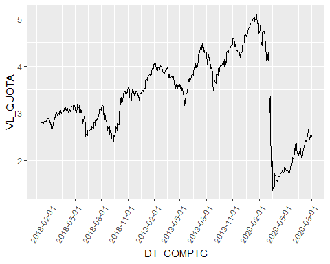

COVID-19 brings a lot of trouble, doesn’t it?

COVID-19帶來很多麻煩，不是嗎？

A financial raw series probably contains some problems in the form of patterns that repeat overtime or according to the economic cycle.

原始金融系列可能包含一些問題，這些問題的形式是重復加班或根據經濟周期。

A daily financial time series commonly has a 5-period seasonality because of the trading days of the week. Some should account for holidays and other days that the financial market does not work. I will omit these cases to simplify the analysis.

由于一周中的交易日，每日財務時間序列通常具有5個周期的季節性。 有些人應該考慮假期以及金融市場無法正常運作的其他日子。 我將省略這些案例以簡化分析。

We can observe in the that the series seems to go upward during a period and down after that. This is a good example of a trend pattern observed in the data.

我們可以觀察到，該系列似乎在一段時間內上升，然后下降。 這是在數據中觀察到的趨勢模式的一個很好的例子。

It is interesting to decompose the series to see “inside” the series and separate each of the effects, to capture the deterministic (trend and seasonality) and the random (remainder) parts of the financial time-series.

分解序列以查看序列“內部”并分離每種影響，以捕獲金融時間序列的確定性(趨勢和季節性)和隨機性(剩余)部分，這很有趣。

分解系列 (Decomposing the series)

A time-series can be decomposed into three components: trend, seasonal, and the remainder (random).

時間序列可以分解為三個部分：趨勢，季節和其余部分(隨機)。

There are two ways that we could do this: The additive form and the multiplicative form.

我們可以通過兩種方式執行此操作：加法形式和乘法形式。

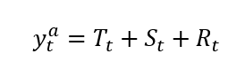
Let y_t be our time-series, T_t represents the trend, S_t is the seasonal component, and R_t is the remainder, or random component.In the additive form, we suppose that the data structure is the sum of its components:

假設y_t是我們的時間序列，T_t代表趨勢，S_t是季節性成分，R_t是余數或隨機成分。以加法形式，我們假設數據結構是其成分之和：

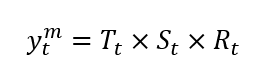
In the multiplicative form, we suppose that the data structure is a product of its components:

以乘法形式，我們假設數據結構是其組成部分的乘積：

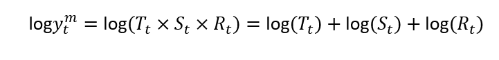
These structures are related. The log of a multiplicative structure is an additive structure of the (log) components:

這些結構是相關的。 乘法結構的對數是(log)組件的加法結構：

Setting a seasonal component of frequency 5, we could account for the weekday effect of the fund returns. We use five because there is no data for the weekends. You also should account for holidays, but since it vary according to the country on analysis, I ignore this effect.

設置頻率為5的季節性成分，我們可以考慮基金收益的平日影響。 我們使用五個，因為沒有周末的數據。 您還應該考慮假期，但是由于分析時會因國家/地區而異，因此我忽略了這種影響。

library(stats) # a package to perform and manipulate time-series objects
 library(lubridate) # a package to work with date objects
 library(TSstudio) # A package to handle time-series data
 
 # getting the starting point of the time-series data
 start_date <- min(alaska$DT_COMPTC)
 
 # The R program does not know that we are working on time-series. So we must tell the software that our data is a time-series. We do this using the ts() function
 
 ## In the ts() function we insert first the vector that has to be handle as a time-series. Second, we tell what is the starting point of the time series. Third, we have to set the frequency of the time-series. In our case, it is 5.
 share_value <- ts(alaska$VL_QUOTA, start =start_date, frequency = 5)
 
 # the function decompose() performs the decomposition of the series. The default option is the additive form.
 dec_sv <- decompose(share_value)
 
 # Take a look!
 plot(dec_sv)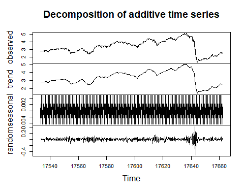

Decomposition of additive time series.

分解附加時間序列。

The above figure shows the complete series observed, and its three components trend, seasonal, and random, decomposed in the additive form.

上圖顯示了觀察到的完整序列，其三個成分趨勢(季節性和隨機)以加法形式分解。

The below figure shows the complete series observed, and its three components trend, seasonal, and random, decomposed in the multiplicative form.

下圖顯示了觀察到的完整序列，其三個分量趨勢(季節性和隨機)以乘法形式分解。

The two forms are very related. The seasonal components change slightly.

兩種形式非常相關。 季節成分略有變化。

dec2_sv <- decompose(share_value, type = "multiplicative")
 
 plot(dec2_sv)

In a time-series application, we are interested in the return of the fund. Another information from the related data set is useless to us.

在時間序列應用程序中，我們對基金的回報感興趣。 來自相關數據集的另一個信息對我們沒有用。

The daily return (Rt) of a fund is obtained from the (log) first difference of the share value. In your data, his variables call VL_QUOTA. The logs are important because give to us a proxy of daily returns in percentage.

基金的日收益率(R t )是從股票價值的(對數)第一差得出的。 在您的數據中，他的變量稱為VL_QUOTA。 日志很重要，因為可以按百分比為我們提供每日收益的代理。

The algorithm for this is:

其算法為：

R1 <- log(alaska$VL_QUOTA)%>% # generate the log of the series
   diff() # take the first difference
 
 plot.ts(R1) # function to plot a time-series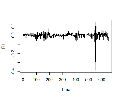

The return (log-first difference) series takes the role of the remainder in the decomposition did before.

返回(對數優先差)序列在之前的分解過程中承擔其余部分的作用。

The random component of the decomposed data is seasonally free. We could do this by hand taking a 5-period difference:

分解后的數據的隨機成分在季節性上不受限制。 我們可以手動進行5個周期的區別：

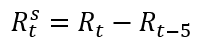
R5 <- R1 %>% diff(lag = 5)
 plot.ts(R5)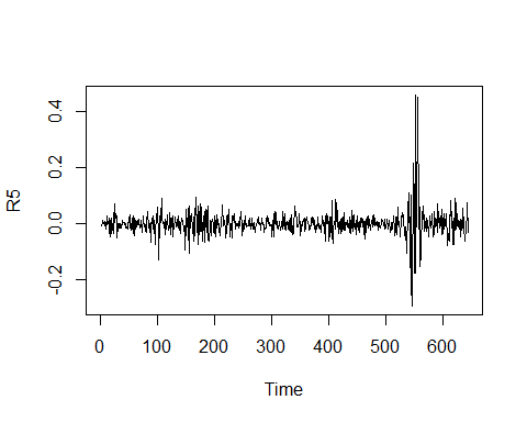

The two graphs are similar. But the second does not have a possible seasonal effect.

這兩個圖是相似的。 但是第二個并沒有可能的季節性影響。

We can plot a graph to identify visually the seasonality of the series using the ggsubseriesplot function of the forecastpackage.

我們可以繪制圖表以使用Forecastpackage的ggsubseriesplot函數直觀地識別系列的季節性。

ggsubseriesplot(share_value)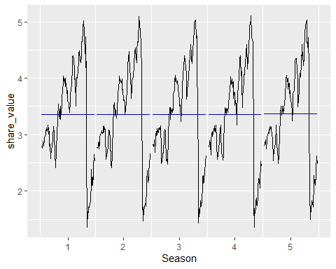

Oh, it seems that our hypothesis for seasonal data was wrong! There is no visually pattern of seasonality in this time-series.

哦，看來我們對季節性數據的假設是錯誤的！ 在此時間序列中，沒有視覺上的季節性模式。

預測 (The Forecasting)

Before forecasting, we have to verify if the data are random or auto-correlated. To verify autocorrelation in the data we can first use the autocorrelation function (ACF) and the partial autocorrelation function (PACF).

進行預測之前，我們必須驗證數據是隨機的還是自動相關的。 為了驗證數據中的自相關，我們可以首先使用自相關函數(ACF)和部分自相關函數(PACF)。

自相關函數和部分自相關函數 (Autocorrelation Function and Partial Autocorrelation Function)

If we use the raw data, the autocorrelation is evident. The blue line indicates that the significance limit of the lag’s autocorrelation. In the below ACF figure, the black vertical line overtaking the horizontal blue line means that the autocorrelation is significant at a 5% confidence level. The sequence of upward lines indicate positive autocorrelation for the tested series.

如果我們使用原始數據，則自相關是明顯的。 藍線表示滯后自相關的顯著性極限。 在下面的ACF圖中，黑色的垂直線超過水平的藍線表示自相關在5％的置信度下很重要。 向上的線序列表示測試序列的正自相關。

To know the order of the autocorrelation, we have to take a look on the Partial Autocorrelation Function (PACF).

要知道自相關的順序，我們必須看一下部分自相關函數(PACF)。

library(TSstudio)
 
 R <- alaska$VL_QUOTA #extract the fund share value from the data
 Racf <- acf(R, lag.max = 12) # compute the ACF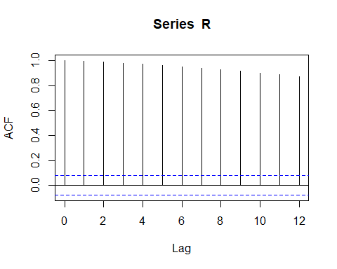

Autocorrelation Function for the fund share value.

基金份額價值的自相關函數。

Rpacf <- pacf(R, lag.max = 12) # compute the PACF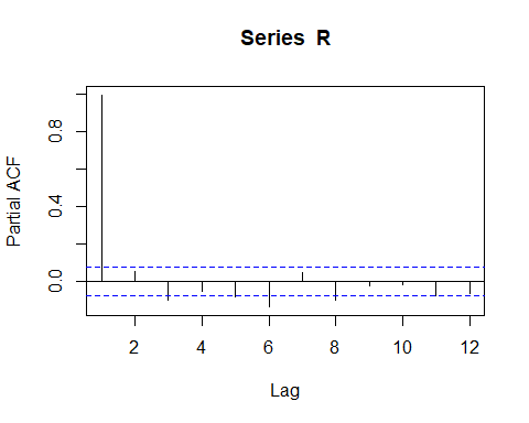

The Partial Autocorrelation Function confirms the autocorrelation in the data for lags 1, 6,and 8.

部分自相關函數可確認數據中的自相關，分別用于滯后1、6和8。

At the most of time, in a financial analysis we are interested on the return of the fund share. To work with it, one can perform the forecasting analysis to the return rather than use the fund share price. I add to you that this procedure is a good way to handle with the non-stationarity of the fund share price.

在大多數時候，在財務分析中，我們對基金份額的回報很感興趣。 要使用它，人們可以對收益進行預測分析，而不必使用基金股票的價格。 我要補充一點，此程序是處理基金股票價格不穩定的好方法。

So, we could perform the (partial) autocorrelation function of the return:

因此，我們可以執行返回的(部分)自相關函數：

library(TSstudio)
 
 Racf <- acf(R1, lag.max = 12) # compute the ACF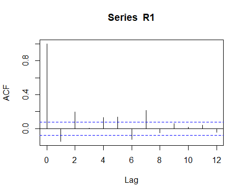

ACF for the fund share (log) Return.

基金份額(日志)收益的ACF。

Racf <- acf(R5, lag.max = 12) # compute the ACF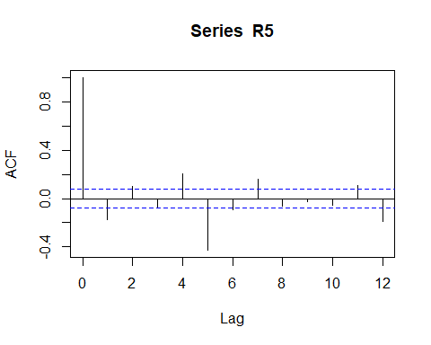

Above ACF figure suggests a negative autocorrelation pattern, but is impossible identify visually the exactly order, or if exists a additional moving average component in the data.

ACF上方的數字表示自相關模式為負，但無法從視覺上確定確切的順序，或者如果數據中存在其他移動平均成分，則無法確定。

Rpacf <- pacf(R1, lag.max = 12) # compute the PACF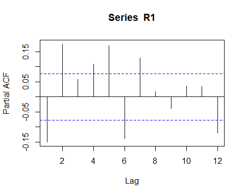

PACF for the fund share (log) Return.

基金份額的PACF(日志)回報。

Rpacf <- pacf(R5, lag.max = 12) # compute the PACF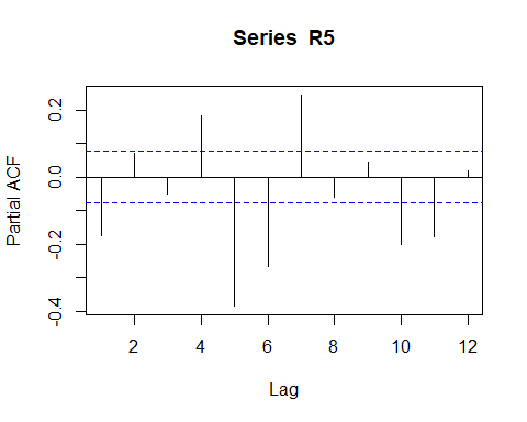

autocorrelation function of the Return does not help us so much. Only that we can set is that exist a negative autucorrelation pattern.

Return的自相關函數對我們沒有太大幫助。 我們唯一可以設置的是存在負的自相關模式。

One way to identify what is the type of components to be used ( autocorrelation or moving average). We could perform various models specifications and choose the model with better AIC or BIC criteria.

一種識別要使用的組件類型(自相關或移動平均值)的方法。 我們可以執行各種模型規范，并選擇具有更好AIC或BIC標準的模型。

使用ARIMA模型進行預測 (Forecasting with ARIMA models)

One good option to perform a forecasting model is to use the family of ARIMA models. For who that is not familiar with theoretical stuff about ARIMA models or even Autocorrelation Functions, I suggest the Brooks books, “Introductory Econometrics for Finance”.

執行預測模型的一個不錯的選擇是使用ARIMA模型系列。 對于那些不熟悉ARIMA模型甚至自相關函數的理論知識的人，我建議使用Brooks的著作“金融計量經濟學入門”。

To model an ARIMA(p,d,q) specification we must to know the order of the autocorrelation component (p), the order of integration (d), and the order of the moving average process (q).

要對ARIMA(p，d，q)規范建模，我們必須知道自相關分量的階數(p)，積分階數(d)和移動平均過程階數(q)。

OK, but, how to do that?

好的，但是，該怎么做呢？

The first strategy is to look to the autocorrelation function and the partial autocorrelation function. since we cant state just one pattern based in what we saw in the graphs, we have to test some model specifications and choose one that have the better AIC or BIC criteria.

第一種策略是考慮自相關函數和部分自相關函數。 由于我們不能根據圖中看到的僅陳述一種模式，因此我們必須測試一些模型規格并選擇一種具有更好的AIC或BIC標準的規格。

We already know that the Returns are stationary, so we do not have to verify stationary conditions (You do it if you don’t trust me :).

我們已經知道退貨是固定的，因此我們不必驗證固定的條件(如果您不信任我，請這樣做：)。

# The ARIMA regression
 arR <- Arima(R5, order = c(1,0,1)) # the auto.arima() function automatically choose the optimal lags to AR and MA components and perform tests of stationarity and seasonality
 
 summary(arR) # now we can see the significant lags## Series: R5 
 ## ARIMA(1,0,1) with non-zero mean 
 ## 
 ## Coefficients:
 ##           ar1     ma1    mean
 ##       -0.8039  0.6604  0.0000
 ## s.e.   0.0534  0.0636  0.0016
 ## 
 ## sigma^2 estimated as 0.001971:  log likelihood=1091.75
 ## AIC=-2175.49   AICc=-2175.43   BIC=-2157.63
 ## 
 ## Training set error measures:
 ##                        ME       RMSE        MAE      MPE     MAPE      MASE
 ## Training set 9.087081e-07 0.04429384 0.02592896 97.49316 192.4589 0.6722356
 ##                     ACF1
 ## Training set 0.005566003

If you want a fast analysis than perform several models and compare the AIC criteria, you could use the auto.arima() functions that automatically choose the orders of autocorrelation, integration and also test for season components in the data.

如果要進行快速分析而不是執行多個模型并比較AIC標準，則可以使用auto.arima()函數自動選擇自相關，積分的順序，并測試數據中的季節成分。

I use it to know that the ARIMA(1,0,1) is the best fit for my data!!

我用它知道ARIMA(1,0,1)最適合我的數據！！

It is interesting to check the residuals to verify if the model accounts for all non random component of the data. We could do that with the checkresiduals function of the forecastpackage.

檢查殘差以驗證模型是否考慮了數據的所有非隨機成分是很有趣的。 我們可以使用Forecastpackage的checkresiduals函數來做到這一點。

checkresiduals(arR)# checking the residuals

 ## 
 ##  Ljung-Box test
 ## 
 ## data:  Residuals from ARIMA(1,0,1) with non-zero mean
 ## Q* = 186.44, df = 7, p-value < 2.2e-16
 ## 
 ## Model df: 3.   Total lags used: 10

Look to the residuals ACF. The model seem to not account for all non-random components, probably by an conditional heteroskedasticity. Since it is not the focus of the post, you could Google for Arch-Garch family models

查看殘差ACF。 該模型似乎沒有考慮到所有非隨機成分，可能是由于條件異方差性造成的。 由于不是本文的重點，因此您可以將Google用于Arch-Garch系列模型

現在，預測！ (Now, the forecasting!)

Forecasting can easily be performed with a single function forecast. You should only insert the model object given by the auto.arima() function and the periods forward to be foreseen.

可以使用單個功能預測輕松進行預測。 您應該只插入由auto.arima()函數給定的模型對象以及可以預見的周期。

farR <-forecast(arR, 15)
 
 ## Fancy way to see the forecasting plot
 
 plot_forecast(farR)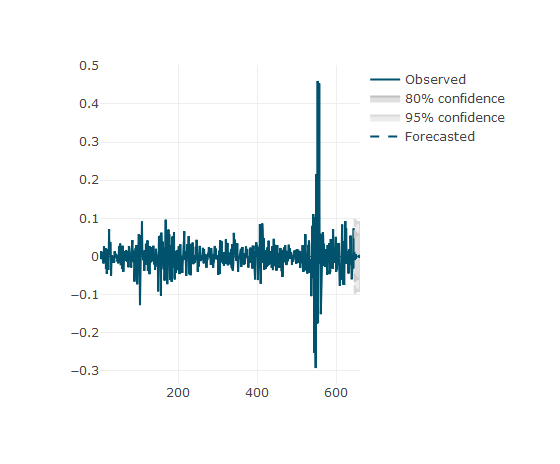

The function plot_forecast of the TSstudio package is a nice way to see the plot forecasting. If you pass the mouse cursor over the plot you cold see the cartesian position of the fund share.

TSstudio軟件包的plot_forecast函數是查看情節預測的好方法。 如果將鼠標指針移到該圖上，您會冷眼看到基金份額的笛卡爾位置。

Now you can go to predict everything that you want. Good luck!

現在，您可以預測所需的一切。 祝好運！