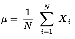
A standard deviation seems like a simple enough concept. It’s a measure of dispersion of data, and is the root of the summed differences between the mean and its data points, divided by the number of data points…minus one to correct for bias.

標準偏差似乎很簡單。 它是對數據分散性的一種度量，是均值與其數據點之和的總和之差除以數據點的數量…… 減去1即可校正偏差 。

This is, I believe, the most oversimplified and maddening concept for any learner, and the intent of this post is to provide a clear and intuitive explanation for Bessel’s Correction, or n-1.

我認為，對于任何學習者來說，這都是最簡單和令人發瘋的概念，這篇文章的目的是為貝塞爾修正(n-1)提供清晰直觀的解釋。

To start, recall the formula for a population mean:

首先，回顧一下總體均值的公式：

What about a sample mean?

樣本的意思是什么？

Well, they look identical, except for the lowercase N. In each case, you just add each x?, and divide by how many x’s there are. If we are dealing with an entire population, we would use N, instead of n, to indicate the total number of points in the population.

好吧，除了小寫字母N之外，它們看起來相同。在每種情況下，您只需將每個x?相加，然后除以x的個數即可。 如果要處理整個總體，則將使用N而不是n來表示總體中的總點數。

Now, what is standard deviation σ (called sigma)?

現在，標準偏差σ是多少？

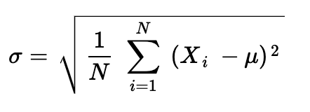
If a population contains N points, then the standard deviation is the square root of the variance, which is the summed-and-averaged squared differences of each data point and the population mean, or μ:

如果總體包含N個點，則標準偏差為方差的平方根，即每個數據點與總體平均值或μ的求和平均值平方差。

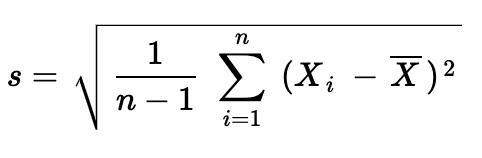
But what about a sample standard deviation, s, with n data points and sample mean x-bar:

但是，具有n個數據點和樣本均值x-bar的樣本標準偏差s呢？

Alas, the dreaded n-1 appears. Why? Shouldn’t it be the same formula? It was virtually the same formula for population mean and sample mean!

,，出現了可怕的n-1。 為什么？ 不應該是相同的公式嗎？ 總體均值和樣本均值實際上是相同的公式！

The short answer is: this is very complex, to such an extent that most instructors explain n-1 by saying the sample standard deviation will ‘a biased estimator’ if you don’t do it.

簡短的答案是： 這非常復雜，以至于大多數教師講n-1時，如果不這樣做，則樣本標準差將成為“有偏估計”。

什么是偏見，為什么存在？ (What is Bias, and Why is it There?)

The Wikipedia explanation can be found here.

Wikipedia的解釋可以在這里找到 。

It’s not helpful.

沒有幫助

To really understand n-1, just like any other brief attempt to explain Bessel’s Correction, requires holding a lot in your head at once. I’m not talking about a proof, either. I’m talking about truly understanding the differences between a sample and a population.

要真正了解N-1，就像任何其他的簡短試圖解釋貝塞爾修正，需要立刻拿著很多在你的頭上。 我也不是在說證明。 我說的是真正了解樣本與總體之間的差異 。

What is a sample?

什么是樣本？

A sample is always a subset of a population it’s intended to represent (a subset can be the same size as the original set, in the unusual case of sampling an entire population without replacement). This is a massive leap alone. Once a sample is taken, there are presumed, hypothetical parameters and distributions built into that sample-representation.

樣品始終是一個人口它意在表示 (一個子集可以是相同大小的原始集合，在沒有更換采樣的整個人口的不尋常的情況下)的子集 。 單單這是一次巨大的飛躍。 抽取樣本后， 該樣本表示中會內置假定的假設參數和分布 。

The very word statistic refers to some piece of information about a sample (such as a mean, or median) which corresponds to some piece of analogous information about the population (again, such as mean, or median) called a parameter. The field of ‘Statistics’ is named as such, instead of ‘Parametrics’, to convey this attitude of inference from smaller to larger, and this leap, again, has many assumptions built into it. For example, if prior assumptions about a sample’s population are actually quantified, this leads to Bayesian statistics. If not, this leads to frequentism, both outside the scope of this post, but nevertheless important angles to consider in the context of Bessel’s correction. (in fact, in Bayesian inference Bessel’s Correction is not used, since prior probabilities about population parameters are intended to handle bias in a different way, upfront. Variance and standard deviation are calculated with plain old n).

統計數據一詞是指有關樣本的某些信息(例如平均值或中位數)，它對應于有關總體的某些類似信息(同樣是平均值或中位數)，稱為參數。 “統計”字段的名稱被這樣命名，而不是“參數”字段，以傳達從小到大的這種推理態度，而這一飛躍又有許多假設。 例如，如果實際量化了關于樣本總體的先前假設，那么這將導致貝葉斯統計 。 如果不是這樣，則會導致頻頻主義 ，這既不在本文討論的范圍之內，也不過是在貝塞爾修正案中要考慮的重要角度。 (實際上，在貝葉斯推斷中未使用Bessel校正，因為有關總體參數的先驗概率旨在以不同的方式預先處理偏差。方差和標準差使用普通old n來計算)。

But let’s not lose focus. Now that we’ve stated the important fundamental difference between a sample and a population, let’s consider the implications of sampling. I will be using the Normal distribution for the following examples for the sake of simplicity, as well as this Jupyter notebook which contains one-million simulated, Normally distributed data points for visualizing intuitions about samples. I highly recommend playing with it yourself, or simply using from sklearn.datasets import make_gaussian_quantiles to get a hands-on feel for what’s really going on with sampling.

但是，我們不要失去重點。 現在，我們已經說明了樣本和總體之間的重要根本區別，讓我們考慮一下樣本的含義。 為簡單起見，我將在以下示例中使用正態分布，以及此Jupyter筆記本 ，其中包含一百萬個模擬的正態分布數據點，用于可視化有關樣本的直覺。 我強烈建議您自己玩，或者只是from sklearn.datasets import make_gaussian_quantiles來獲得對采樣實際操作的親身體驗。

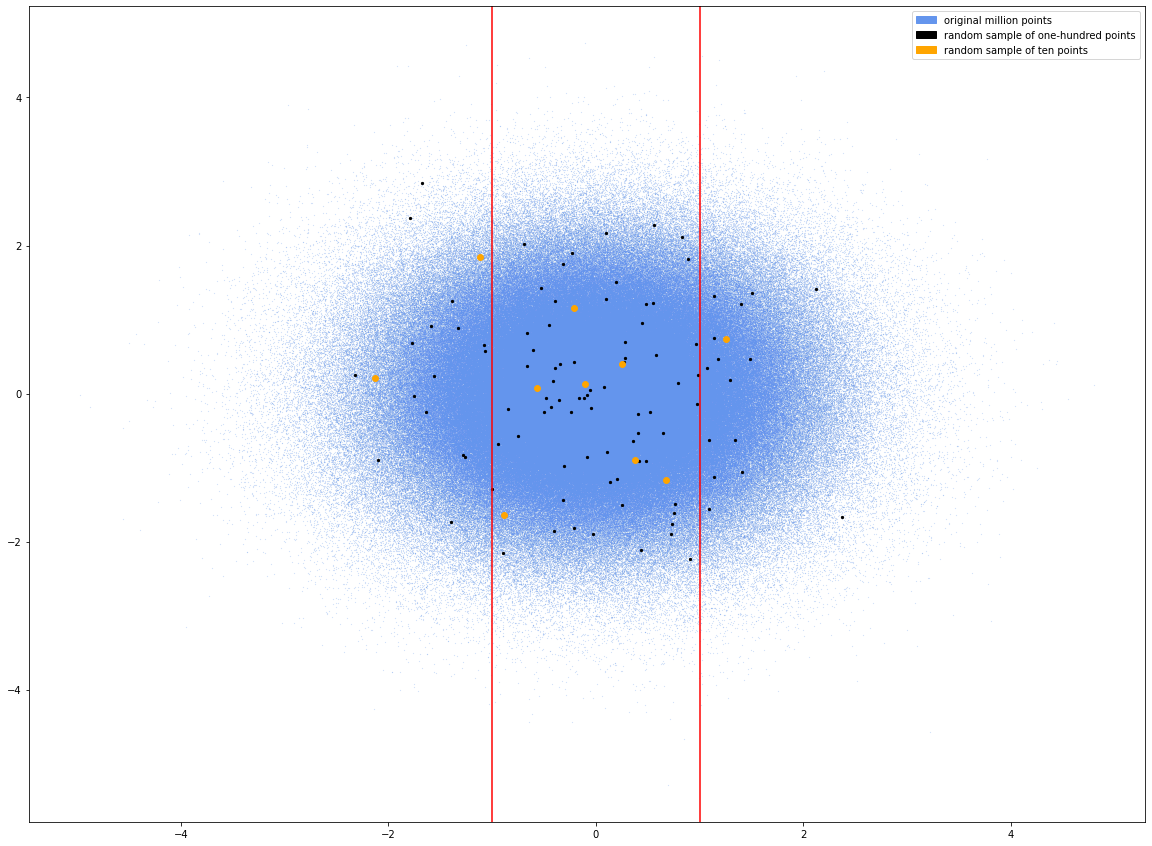
Here is an image of one million randomly-generated, Normally distributed points. We will call it our population:

這是一百萬個隨機生成的正態分布點的圖像。 我們稱其為人口：

To further simplify things, we will only be considering mean, variance, standard deviation, etc., based on the x-values. (That is, I could have used a mere number line for these visualizations, but having the y-axis more effectively displays the distribution across the x axis).

為了進一步簡化，我們將僅基于x值考慮均值，方差，標準差等。 (也就是說，我本可以僅使用數字線進行這些可視化，但是使y軸更有效地顯示x軸上的分布)。

This is a population, so N = 1,000,000. It’s Normally distributed, so the mean is 0.0, and the standard deviation is 1.0.

這是人口，因此N = 1,000,000。 它是正態分布的，因此平均值為0.0，標準偏差為1.0。

I took two random samples, the first only 10 points and the second 100 points:

我隨機抽取了兩個樣本，前一個僅10分，第二個100分：

Now, let’s take a look at these two samples, without and with Bessel’s Correction, along with their standard deviations (biased and unbiased, respectively). The first sample is only 10 points, and the second sample is 100 points.

現在，讓我們看一下這兩個樣本(不帶貝塞爾校正和不帶貝塞爾校正)以及它們的標準偏差(分別為有偏和無偏)。 第一個樣本僅為10分，第二個樣本為100分。

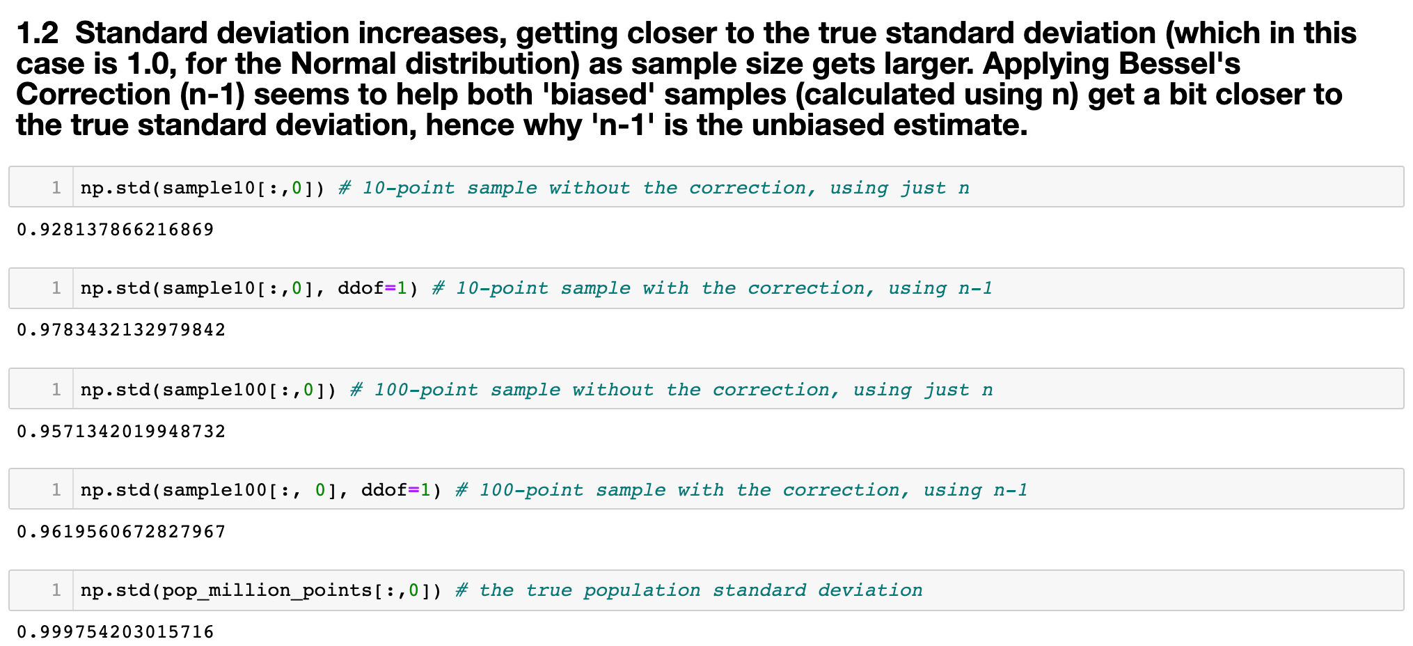
Take a good long look at the above image. Bessel’s Correction does seem to be helping. It makes sense: very often the sample standard deviation will be lower than the population standard deviation, especially if the sample is small, because unrepresentative points (‘biased’ points, i.e. farther from the mean) will have more of an impact on the calculation of variance. Because the difference between each data point and the sample mean is being squared, the range of possible differences will be smaller than the real range if the population mean was used. Furthermore, taking a square root is a concave function, and therefore introduces ‘downward bias’ in estimations.

請仔細看一下上面的圖片。 貝塞爾的矯正似乎確實有所幫助。 這是有道理的：樣本標準偏差通常會低于總體標準偏差，尤其是在樣本較小的情況下，因為不具有代表性的點(“有偏點”，即距離均值較遠)會對計算產生更大的影響差異。 由于每個數據點和樣本均值之間的差異均被平方，因此，如果使用總體均值，則可能的差異范圍將小于實際范圍。 此外， 取平方根是一個凹函數，因此在估計中引入了“向下偏差” 。

Another way of thinking about it is this: the larger your sample, the more of an opportunity you have to run into more population-representative points, i.e. points that are close to the mean. Therefore, you have less of a chance of getting a sample mean which results in differences which are too small, leading to a too-small variance, and you’re left with an undershot standard deviation.

另一種思考方式是：樣本越大， 就越有機會碰到更多具有人口代表性的點，即接近均值的點。 因此，您獲得樣本均值的機會較小，樣本均值導致的差異過小，導致方差過小，并且留下的標準偏差不足。

On average, samples of a Normally-distributed population will produce a variance which is biased downward by a factor of n-1 on average. (Incidentally, I believe the distribution of sample biases themselves are described by Student’s t-distribution, determined by n). Therefore, by dividing the square-rooted variance by n-1, we make the denominator smaller, thereby making the result larger and leading to a so-called ‘unbiased’ estimate.

平均而言，正態分布總體的樣本將產生方差，該方差平均向下降低n-1倍 。 (順便說一句，我相信樣本偏差本身的分布由Student的t分布描述，由n確定)。 因此，通過將平方根方差除以n-1，我們使分母變小，從而使結果變大，從而導致所謂的“無偏”估計。

The key point to emphasize here is that Bessel’s Correction, or dividing by n-1, doesn’t always actually help! Because the potential sample-variances are themselves t-distributed, you will unwittingly run into cases where n-1 will overshoot the real population standard deviation. It just so happens that n-1 is the best tool we have to correct for bias most of the time.

這里要強調的關鍵是，貝塞爾校正或除以n-1并不一定總是有幫助！ 因為潛在的樣本方差本身是t分布的，所以您會無意中遇到n-1會超出實際總體標準差的情況。 碰巧的是，n-1是大多數時候我們必須校正偏差的最佳工具 。

To prove this, check out the same Jupyter notebook where I’ve merely changed the random seed until I found some samples whose standard deviation was already close to the population standard deviation, and where n-1 added more bias:

為了證明這一點，請查看我只更改了隨機種子的同一本Jupyter筆記本 直到我發現一些標準偏差已經接近總體標準偏差的樣本，并且其中n-1 增加了更多偏差 ：

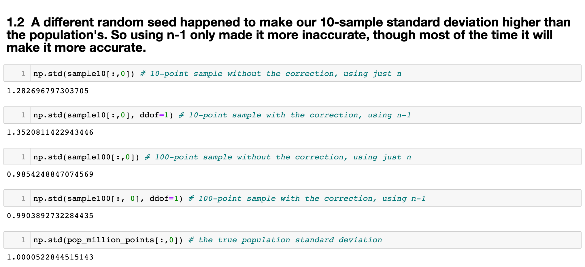
In this case, Bessel’s Correction actually hurt us!

在這種情況下，貝塞爾的更正實際上傷害了我們！

Thus, Bessel’s Correction is not always a correction. It’s called such because most of the time, when sampling, we don’t know the population parameters. We don’t know the real mean or variance or standard deviation. Thus, we are relying on the fact that because we know the rate of bad luck (undershooting, or downward bias), we can counteract bad luck by the inverse of that rate: n-1.

因此，貝塞爾的校正并不總是校正。 之所以這樣稱呼，是因為在大多數情況下，抽樣時我們不知道總體參數 。 我們不知道真實的均值或方差或標準差。 因此，我們依靠這樣一個事實， 因為我們知道厄運率(下沖或向下偏差)，因此可以通過該比率的倒數來抵消厄運：n-1。

But what if you get lucky? Just like in the cells above, this can happen sometimes. Your sample can occasionally produce the correct standard deviation, or even overshoot it, in which case n-1 ironically adds bias.

但是，如果您幸運的話，該怎么辦？ 就像上面的單元格一樣，有時可能會發生這種情況。 您的樣品有時可能會產生正確的標準偏差，甚至會產生超標，在這種情況下，n-1具有諷刺意味的是會增加偏差。

Nevertheless, it’s the best tool we have for bias correction in a state of ignorance. The need for bias correction doesn’t exist from a God’s-eye point of view, where the parameters are known.

但是，它是我們在無知狀態下進行偏差校正的最佳工具。 從參數已知的角度來看，不存在偏差校正的需要。

At the end of the day, this fundamentally comes down to understanding the crucial difference between a sample and a population, as well as why Bayesian Inference is such a different approach to classical problems, where guesses about the parameters are made upfront via prior probabilities, thus removing the need for Bessel’s Correction.

歸根結底，這從根本上歸結為理解樣本與總體之間的關鍵差異，以及為什么貝葉斯推理是對古典問題的如此不同的方法，其中對參數的猜測是通過先驗概率預先做出的 ，從而消除了貝塞爾校正的需要。

I’ll focus on Bayesian statistics in future posts. Thanks for reading!

在以后的文章中，我將重點介紹貝葉斯統計。 謝謝閱讀！