Welcome back to my 100 Days of Data Science Challenge Journey. On day 4 and 5, I work on TMDB Box Office Prediction Dataset available on Kaggle.

歡迎回到我的100天數據科學挑戰之旅。 在第4天和第5天，我將研究Kaggle上提供的TMDB票房預測數據集。

I’ll start by importing some useful libraries that we need in this task.

我將從導入此任務中需要的一些有用的庫開始。

import pandas as pd# for visualizations
import matplotlib.pyplot as plt
import seaborn as sns
%matplotlib inline
plt.style.use('dark_background')

數據加載與探索 (Data Loading and Exploration)

Once you downloaded data from the Kaggle, you will have 3 files. As this is a prediction competition, you have train, test, and sample_submission file. For this project, my motive is only to perform data analysis and visuals. I am going to ignore test.csv and sample_submission.csv files.

從Kaggle下載數據后，您將擁有3個文件。 由于這是一場預測比賽，因此您具有訓練，測試和sample_submission文件。 對于這個項目，我的動機只是執行數據分析和視覺效果。 我將忽略test.csv和sample_submission.csv文件。

Let’s load train.csv in data frame using pandas.

讓我們使用熊貓在數據框中加載train.csv。

%time train = pd.read_csv('./data/tmdb-box-office-prediction/train.csv')# output
CPU times: user 258 ms, sys: 132 ms, total: 389 ms
Wall time: 403 ms

關于數據集： (About the dataset:)

id: Integer unique id of each moviebelongs_to_collection: Contains the TMDB Id, Name, Movie Poster, and Backdrop URL of a movie in JSON format.budget: Budget of a movie in dollars. Some row contains 0 values, which mean unknown.genres: Contains all the Genres Name & TMDB Id in JSON Format.homepage: Contains the official URL of a movie.imdb_id: IMDB id of a movie (string).original_language: Two-digit code of the original language, in which the movie was made.original_title: The original title of a movie in original_language.overview: Brief description of the movie.popularity: Popularity of the movie.poster_path: Poster path of a movie. You can see full poster image by adding URL after this link → https://image.tmdb.org/t/p/original/production_companies: All production company name and TMDB id in JSON format of a movie.production_countries: Two-digit code and the full name of the production company in JSON format.release_date: The release date of a movie in mm/dd/yy format.runtime: Total runtime of a movie in minutes (Integer).spoken_languages: Two-digit code and the full name of the spoken language.status: Is the movie released or rumored?tagline: Tagline of a movietitle: English title of a movieKeywords: TMDB Id and name of all the keywords in JSON format.cast: All cast TMDB id, name, character name, gender (1 = Female, 2 = Male) in JSON formatcrew: Name, TMDB id, profile path of various kind of crew members job like Director, Writer, Art, Sound, etc.revenue: Total revenue earned by a movie in dollars.

Let’s have a look at the sample data.

讓我們看一下樣本數據。

train.head()

As we can see that some features have dictionaries, hence I am dropping all such columns for now.

如我們所見，某些功能具有字典，因此我暫時刪除所有此類列。

train = train.drop(['belongs_to_collection', 'genres', 'crew',
'cast', 'Keywords', 'spoken_languages', 'production_companies', 'production_countries', 'tagline','overview','homepage'], axis=1)

Now it time to have a look at statistics of the data.

現在該看一下數據統計了。

print("Shape of data is ")
train.shape# OutputShape of data is
(3000, 12)

Dataframe information.

數據框信息。

train.info()# Output
<class 'pandas.core.frame.DataFrame'>
RangeIndex: 3000 entries, 0 to 2999
Data columns (total 12 columns):
 #   Column             Non-Null Count  Dtype  
---  ------             --------------  -----  
 0   id                 3000 non-null   int64  
 1   budget             3000 non-null   int64  
 2   imdb_id            3000 non-null   object 
 3   original_language  3000 non-null   object 
 4   original_title     3000 non-null   object 
 5   popularity         3000 non-null   float64
 6   poster_path        2999 non-null   object 
 7   release_date       3000 non-null   object 
 8   runtime            2998 non-null   float64
 9   status             3000 non-null   object 
 10  title              3000 non-null   object 
 11  revenue            3000 non-null   int64  
dtypes: float64(2), int64(3), object(7)
memory usage: 281.4+ KB

Describe dataframe.

描述數據框。

train.describe()

Let’s create new columns for release weekday, date, month, and year.

讓我們為發布工作日，日期，月份和年份創建新列。

train['release_date'] = pd.to_datetime(train['release_date'], infer_datetime_format=True)train['release_day'] = train['release_date'].apply(lambda t: t.day)train['release_weekday'] = train['release_date'].apply(lambda t: t.weekday())train['release_month'] = train['release_date'].apply(lambda t: t.month)
train['release_year'] = train['release_date'].apply(lambda t: t.year if t.year < 2018 else t.year -100)

數據分析與可視化 (Data Analysis and Visualization)

問題1：哪部電影的收入最高？ (Question 1: Which movie made the highest revenue?)

train[train['revenue'] == train['revenue'].max()]

train[['id','title','budget','revenue']].sort_values(['revenue'], ascending=False).head(10).style.background_gradient(subset='revenue', cmap='BuGn')# Please note that output has a gradient style, but in a medium, it is not possible to show.

The Avengers movie has made the highest revenue.

復仇者聯盟電影的收入最高。

問題2：哪部電影的預算最高？ (Question 2 : Which movie has the highest budget?)

train[train['budget'] == train['budget'].max()]

train[['id','title','budget', 'revenue']].sort_values(['budget'], ascending=False).head(10).style.background_gradient(subset=['budget', 'revenue'], cmap='PuBu')

Pirates of the Caribbean: On Stranger Tides is most expensive movie.

加勒比海盜：驚濤怪浪是最昂貴的電影。

問題3：哪部電影是最長的電影？ (Question 3: Which movie is longest movie?)

train[train['runtime'] == train['runtime'].max()]

plt.hist(train['runtime'].fillna(0) / 60, bins=40);
plt.title('Distribution of length of film in hours', fontsize=16, color='white');
plt.xlabel('Duration of Movie in Hours')
plt.ylabel('Number of Movies')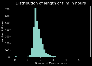

train[['id','title','runtime', 'budget', 'revenue']].sort_values(['runtime'],ascending=False).head(10).style.background_gradient(subset=['runtime','budget','revenue'], cmap='YlGn')

Carlos is the longest movie, with 338 minutes (5 hours and 38 minutes) of runtime.

卡洛斯(Carlos)是最長的電影，有338分鐘(5小時38分鐘)的運行時間。

問題4：大多數電影在哪一年發行的？ (Question 4: In which year most movies were released?)

plt.figure(figsize=(20,12))
edgecolor=(0,0,0),
sns.countplot(train['release_year'].sort_values(), palette = "Dark2", edgecolor=(0,0,0))
plt.title("Movie Release count by Year",fontsize=20)
plt.xlabel('Release Year')
plt.ylabel('Number of Movies Release')
plt.xticks(fontsize=12,rotation=90)
plt.show()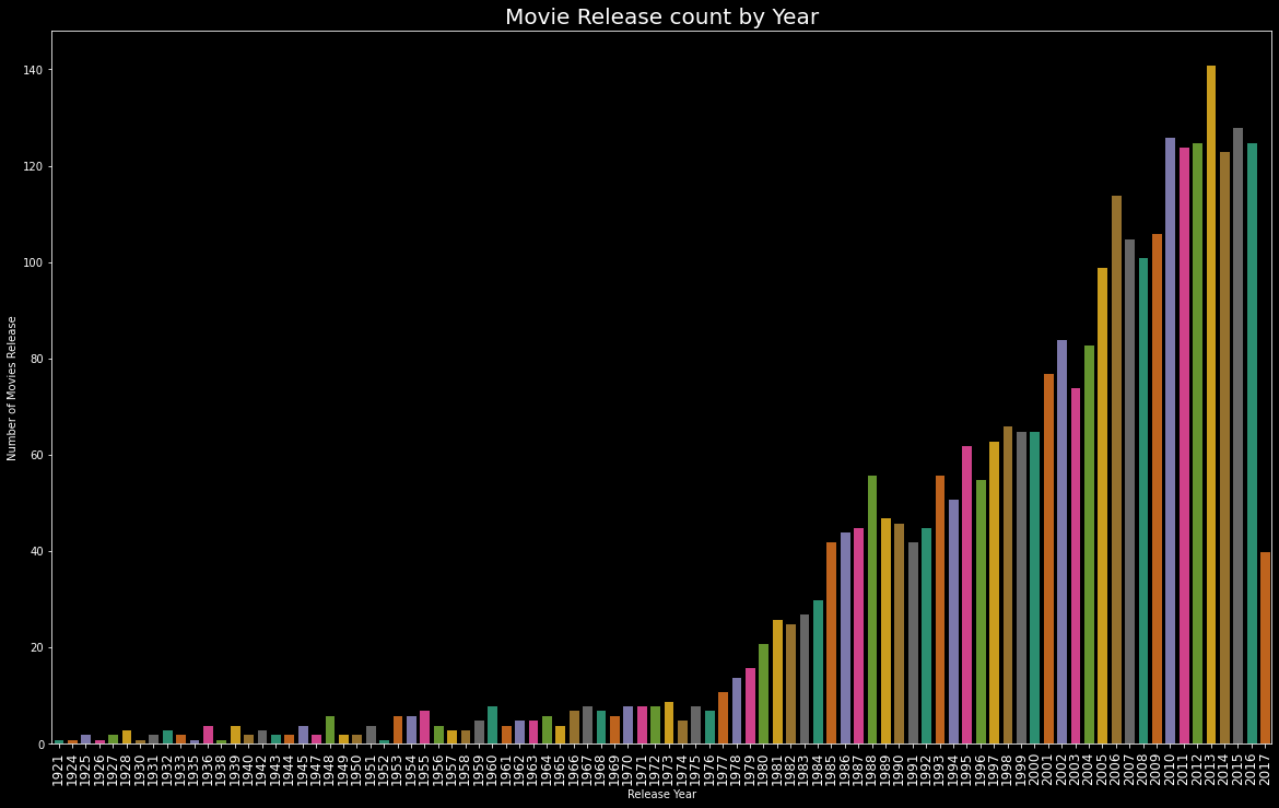

train['release_year'].value_counts().head()# Output2013    141
2015    128
2010    126
2016    125
2012    125
Name: release_year, dtype: int64

In 2013 total 141 movies were released.

2013年，總共發行了141部電影。

問題5：最受歡迎和最低人氣的電影。 (Question 5 : Movies with Highest and Lowest popularity.)

Most popular Movie:

最受歡迎的電影：

train[train['popularity']==train['popularity'].max()][['original_title','popularity','release_date','revenue']]

Least Popular Movie:

最不受歡迎的電影：

train[train['popularity']==train['popularity'].min()][['original_title','popularity','release_date','revenue']]

Lets create popularity distribution plot.

讓我們創建人氣分布圖。

plt.figure(figsize=(20,12))
edgecolor=(0,0,0),
sns.distplot(train['popularity'], kde=False)
plt.title("Movie Popularity Count",fontsize=20)
plt.xlabel('Popularity')
plt.ylabel('Count')
plt.xticks(fontsize=12,rotation=90)
plt.show()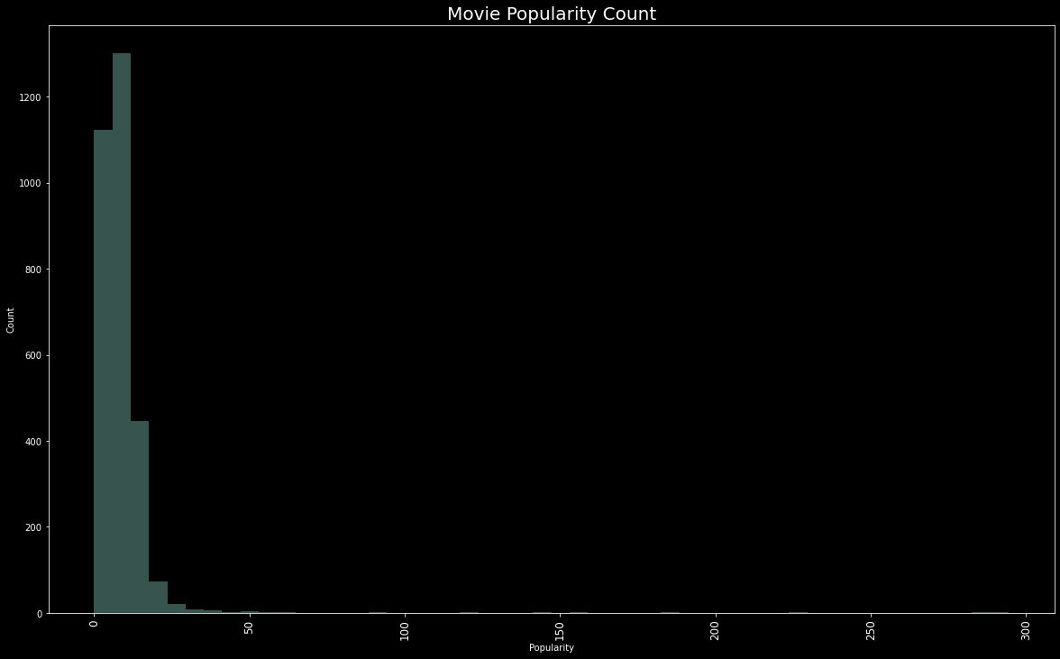

Wonder Woman movie have highest popularity of 294.33 whereas Big Time movie have lowest popularity which is 0.

《神奇女俠》電影的最高人氣為294.33，而《大時代》電影的最低人氣為0。

問題6：從1921年到2017年，大多數電影在哪個月發行？ (Question 6 : In which month most movies are released from 1921 to 2017?)

plt.figure(figsize=(20,12))
edgecolor=(0,0,0),
sns.countplot(train['release_month'].sort_values(), palette = "Dark2", edgecolor=(0,0,0))
plt.title("Movie Release count by Month",fontsize=20)
plt.xlabel('Release Month')
plt.ylabel('Number of Movies Release')
plt.xticks(fontsize=12)
plt.show()

train['release_month'].value_counts()# Output
9     362
10    307
12    263
8     256
4     245
3     238
6     237
2     226
5     224
11    221
1     212
7     209
Name: release_month, dtype: int64

In september month most movies are relesed which is around 362.

在9月中，大多數電影都已發行，大約362。

問題7：大多數電影在哪個月上映？ (Question 7 : On which date of month most movies are released?)

plt.figure(figsize=(20,12))
edgecolor=(0,0,0),
sns.countplot(train['release_day'].sort_values(), palette = "Dark2", edgecolor=(0,0,0))
plt.title("Movie Release count by Day of Month",fontsize=20)
plt.xlabel('Release Day')
plt.ylabel('Number of Movies Release')
plt.xticks(fontsize=12)
plt.show()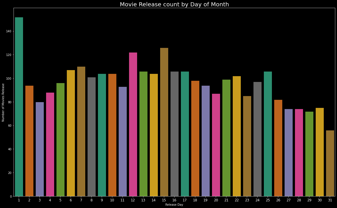

train['release_day'].value_counts().head()#Output
1     152
15    126
12    122
7     110
6     107
Name: release_day, dtype: int64

首次發布影片的最高數量為152。 (On first date highest number of movies are released, 152.)

問題8：大多數電影在一周的哪一天發行？ (Question 8 : On which day of week most movies are released?)

plt.figure(figsize=(20,12))
sns.countplot(train['release_weekday'].sort_values(), palette='Dark2')
loc = np.array(range(len(train['release_weekday'].unique())))
day_labels = ['Mon', 'Tue', 'Wed', 'Thu', 'Fri', 'Sat', 'Sun']
plt.xlabel('Release Day of Week')
plt.ylabel('Number of Movies Release')
plt.xticks(loc, day_labels, fontsize=12)
plt.show()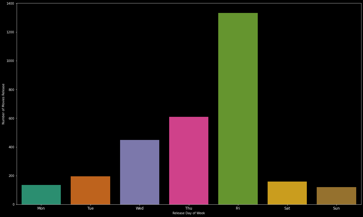

train['release_weekday'].value_counts()# Output
4    1334
3     609
2     449
1     196
5     158
0     135
6     119
Name: release_weekday, dtype: int64

星期五上映的電影數量最多。 (Highest number of movies released on friday.)

最后的話 (Final Words)

I hope this article was helpful to you. I tried to answer a few questions using data science. There are many more questions to ask. Now, I will move towards another dataset tomorrow. All the codes of data analysis and visuals can be found at this GitHub repository or Kaggle kernel.

希望本文對您有所幫助。 我嘗試使用數據科學回答一些問題。 還有更多問題要問。 現在，我明天將移至另一個數據集。 可以在此GitHub存儲庫或Kaggle內核中找到所有數據分析和可視化代碼。

Thanks for reading.

謝謝閱讀。

I appreciate any feedback.

我感謝任何反饋。

數據科學進展100天 (100 Days of Data Science Progress)

If you like my work and want to support me, I’d greatly appreciate it if you follow me on my social media channels:

如果您喜歡我的工作并希望支持我，那么如果您在我的社交媒體頻道上關注我，我將不勝感激：

• The best way to support me is by following me on Medium.

  支持我的最佳方法是在Medium上關注我。

• Subscribe to my new YouTube channel.

  訂閱我的新YouTube頻道 。

• Sign up on my email list.

  在我的電子郵件列表中注冊。