DL DATATHON- AI4Impact

DL DATATHON- AI4影響

Published by Team AI Traders — Suyash Lohia, Nguyen Khoi Phan, Nikunj Taneja, Naman Agarwal and Mihir Gupta

AI交易員團隊發布 -Suyash Lohia，Nguyen Khoi Phan，Nikonj Taneja，Naman Agarwal和Mihir Gupta

介紹 (Introduction)

Most sources of energy that are of renewable nature are reliant on the environment. The production of wind energy is largely dependent on the wind speed and its direction. A simple, yet integral concept that is necessary for the production of wind energy is the blowing of the wind. Hence, producing energy is only possible, when wind blows.

大部分具有可再生性質的能源都依賴于環境。 風能的產生在很大程度上取決于風速及其方向。 產生風能所必需的一個簡單但不可或缺的概念就是吹風。 因此，只有在風吹動時才可能產生能量。

Wind energy as a renewable source of energy is an extremely clean fuel source since it causes very minimal air pollution contrary to the power plants that are reliant on the combustion of fossil fuels such as coal and natural gas. Additionally, due its clean property, wind energy production is a rather safe process since it does not involve the emission of any hazardous gasses. However, despite the various benefits of using wind energy, it is an unfavourable source. Wind energy production’s heavy dependence on the environment causes wind energy to be of an unpredictable nature as compared to non renewable sources of energy such as fossil fuels and nuclear energy.

風能作為一種可再生能源是一種非常清潔的燃料，因為它與依賴煤和天然氣等化石燃料燃燒的發電廠相反，它造成的空氣污染極少。 此外，由于其清潔特性，風能生產是一個相當安全的過程，因為它不涉及任何有害氣體的排放。 但是，盡管使用風能有許多好處，但它是不利的來源。 與不可再生的能源(如化石燃料和核能)相比，風能生產對環境的嚴重依賴導致風能具有不可預測的性質。

利益相關者分析 (Stakeholder Analysis)

Wind energy production primarily consists of three core stakeholders. They are collectively accountable for establishing the production line for wind energy. The three key stakeholders are:

風能生產主要由三個核心利益相關者組成。 他們共同負責建立風能生產線。 三個主要利益相關者是：

Energy traders: these are companies which help predict and trade many aspects of energy, including the expected production of wind energy. In this project, the role of the energy trader is to help solve the shortfall through financial instruments.

能源貿易商 ：這些公司可以幫助預測和交易能源的許多方面，包括風能的預期產量。 在該項目中，能源交易員的作用是通過金融工具幫助解決短缺問題。

Wind energy producers: These refer to the companies that manage and operate wind farms. They act as the intermediary between the grid operators and the energy traders, thereby selling the energy they produce to the Grid Operators.

風能生產商 ：這些是指管理和運營風電場的公司。 它們充當電網運營商和能源貿易商之間的中介，從而將他們生產的能源出售給電網運營商。

Grid Operators: These refer to the various companies bestowed with the responsibility to manage the power grids over a nation or region for a given country or region. They buy pre-determined blocks of energy (measured in kWh) from the wind energy producers.

電網運營商：這些是指賦予特定國家或地區管理一個國家或地區電網的各種公司。 他們從風能生產商那里購買了預定的能量塊(以千瓦時為單位)。

In principle, the role of the grid operators is to create a steady supply of electrical energy for the society. In fact, in cases of power outages or shortages, the government is liable to fine grid operators. In turn, this risk further percolates down to the energy traders and wind energy producers who are held responsible for the issues arising and are further made accountable to compensate for the shortfalls and the fines charged.

原則上，電網運營商的作用是為社會創造穩定的電能供應。 實際上，在停電或短缺的情況下，政府有責任對電網經營者處以罰款。 反過來，這種風險會進一步滲透到能源貿易商和風能生產商，他們對所出現的問題負責，并進一步承擔責任，以彌補不足和罰款。

Problem Statement: Having understood the relationship between the various stakeholders in the process of wind energy production and its lead up to the marketplace, it is essential to understand the problem at hand. In the aforementioned setup, the wind energy producers forecast the energy they will produce in the future to the grid. This forecast is understood as a promissory minimum that the grid would expect from the energy producers. Differences in the actual energy produced in an interval in comparison with the forecast could be of two types:

問題陳述：在了解風能生產過程中各個利益相關者之間的關系以及將風能推向市場之前，了解當前的問題至關重要。 在上述設置中，風能生產商預測未來將向電網生產的能源。 該預測被理解為電網對能源生產商的期望下限。 間隔內產生的實際能量與預測值之間的差異可能有兩種：

1. Shortfall — The scenario where the actual energy produced is lesser than the forecast. When this happens, the grid receives a fine from the wind energy producer.

   短缺—實際產生的能量小于預測的情況。 發生這種情況時，電網將從風能生產商處罰款。

2. Excess — The scenario where the actual energy produced is greater than the forecast. When this happens, there is no direct fine, however, the wind energy producers do not receive any compensation for the excess energy produced.

   多余 -實際產生的能量大于預測的情況。 發生這種情況時，不會直接處以罰款，但是，風能生產者不會就產生的多余能量獲得任何補償。

Our role as the energy trader is to provide service to our client, the wind producer in 2 ways:

我們作為能源貿易商的角色是通過兩種方式向我們的客戶(風能生產商)提供服務：

1. Create the forecast for the wind producers to be handed to the grid.
   創建將要移交給電網的風力發電商的預測。
2. Purchase overpriced energy from the spot market and provide it to the grid in the event of a shortfall.
   從現貨市場購買價格過高的能源，并在出現短缺時將其提供給電網。

Objective

目的

In the capacity of energy traders, we were required to get hourly T+18 hour energy forecasts for energy production which would then be passed on the energy producers. In light of this, the main objective of the task was to maximise profits While doing so,

以能源貿易商的身份，我們被要求獲得每小時T + 18小時的能源生產能源預測，然后將其傳遞給能源生產商。 有鑒于此，任務的主要目標是實現利潤最大化。

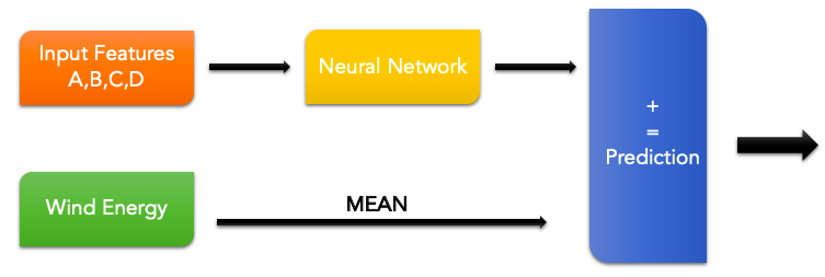
Our objective in this project is to play the role of an energy trader. To simplify the problem, the trading algorithm (described below) is fixed and cannot be altered. Your goal is to get a T+18 hour energy forecast, every hour. The objective is to maximise profits for your client using your energy production forecast and the given trading algorithm.

我們在該項目中的目標是扮演能源貿易商的角色。 為了簡化問題，交易算法(如下所述)是固定的，不能更改。 您的目標是每小時獲得T + 18小時的能源預測。 目的是使用您的能源產量預測和給定的交易算法為您的客戶最大化利潤。

交易設置的更深層次的復雜性： (Deeper Intricacies of the Trading Setup:)

In line with the aforementioned objective, we were required to make a T+18 hour hour forecast of the energy for our client’s wind farms. As per the simulated set-up, our client was to be paid 10 euro cents/kWh sold to the grid. However, the sale of the energy units were subject to certain conditions. We would only sell to the grid operators, what we in the capacity of energy traders forecasted for that particular day and if our forecast was below the actual energy production, then we were liable to buy the deficit from the spot market at the rate of 20 euro cents/kWh. On the other hand, if the actual energy production exceeded the forecast then the excess would be observed by the grid, without the grid operator (i.e. our client) being compensated for the excess.

根據上述目標，我們被要求對客戶風電場的能源進行T + 18小時的預測。 根據模擬設置，向客戶出售給電網的價格為10歐分/ kWh。 但是，出售能源單位要遵守某些條件。 我們只會向電網運營商出售該天在能源交易員的預測中所能達到的水平，如果我們的預測低于實際的能源產量，則我們有責任以20的比率從現貨市場購買赤字。歐分/ kWh。 另一方面，如果實際的能源產量超過了預測，那么電網將觀察到過量，而電網運營商(即我們的客戶)將無法獲得補償。

As for the time scales involved, the first 18 hours (also termed as the warmup period) were deemed void — such that no trades were to be performed during this period. After the warm-up period, we were expected to produce a T+18 hour forecast for the energy production, every hour. Furthermore, this trading period was to continue over weekends and public holidays which would end at the end of the evaluation period.

至于所涉及的時間尺度，最初的18個小時(也稱為預熱期)被認為是無效的，因此在此期間不得進行任何交易。 在預熱期之后，我們預計每小時會產生T + 18小時的能源生產預測。 此外，該交易期將持續到周末和公共假日，直到評估期結束。

As a part of the project, we will compare the actual energy produced with the forecast we prepare on an hourly basis. In the event of the forecast being equal or lesser than the actual energy produced (excess), we are paid 10 euro cents per kWh. This amount is added to our cash at hand, increasing its positive balance. If, in case our cash at hand balance turned negative, we would have to settle our debt(accumulated negative balance) before receiving the amount from the grid. As mentioned previously, excess production over the forecast is not compensated.

作為項目的一部分，我們將每小時產生的實際能量與我們準備的預測進行比較。 如果預測值等于或小于實際產生的能量(過量)，我們將為每度電支付10歐分。 這筆款項將添加到我們的手頭現金中，從而增加其正余額。 如果在手頭現金余額變為負數的情況下，我們必須先償還債務(累計負余額)，然后才能從電網接收金額。 如前所述，超出預測的過剩產量將不予補償。

Contrarily, if there happens to be a shortfall we will have to ensure supplying the promised forecast to the grid by purchasing the shortfall at an overpriced rate from the spot market. Naturally, our cash at hand balance has to be positive for us to make purchases from the spot market. However, if this is not the case, we will be fined 100 euro cents per kWh for the amount of shortfall, which further gets added to our cumulative debt.

相反，如果碰巧出現短缺，我們將必須通過從現貨市場以過高的價格購買短缺來確保將承諾的預測提供給電網。 當然，我們的手頭現金余額對我們來說必須是正數，以便我們從現貨市場購買商品。 但是，如果不是這種情況，我們將對不足額度每千瓦時罰款100歐分，這進一步加重了我們的累積債務。

We were given a sum of 10,000,000 Euro-cents as part of our ‘cash at hand’ at the start and were required to return this amount at the end of the evaluation period, alongside the remainder which were to be our client’s profits.

我們一開始就獲得了10,000,000歐分作為“手頭現金”的一部分，并被要求在評估期結束時返還這筆款項，其余部分將作為客戶的利潤。

數據集： (Datasets:)

In this project we have used two main datasets:

在這個項目中，我們使用了兩個主要的數據集：

1. Wind Energy Production: The source that we have used to obtain data on wind energy production is the French energy transmission authority, Réseau de transport d’électricité (RTE). We have used near real time data, standardised and averaged to 1 hour. The data used is for the period of Jan 2017 — present, with the data represented in kWh. As the dataset comprises wind production data for the Ile-de-France near Paris, it has been named energy-ile-de-france.

   風能生產：我們用于獲取風能生產數據的來源是法國能源傳輸機構Réseaude transport d'électricité(RTE)。 我們使用了近實時數據，經過標準化，平均時間為1小時。 所使用的數據為2017年1月至今的數據，以kWh表示。 由于數據集包含巴黎附近法蘭西島的風力生產數據，因此已被命名為ile-france。

2. Wind Forecasts: In addition to the Wind energy production data, we were provided with wind forecasts in 8 locations in the Ile-de-France region, with each location representing a key wind farm. Similar to the production data, the forecast data is from January 2017 to the present.The wind forecast data has been taken from two different wind models, each of which studies two variables, wind speed and direction. The wind speed has been represented in m/s and direction as a bearing in degrees. The data is interpolated to the base of 1 hour and is updated 4 times on a daily basis. The data has been obtained from Terra Weather.

   風力預報：除了風力發電量數據，我們還為法蘭西島地區的8個地點提供了風力預報，每個地點代表一個關鍵的風力發電場。 與生產數據類似，天氣預報數據為2017年1月至今的數據。天氣預報數據來自兩個不同的風模型，每個模型研究兩個變量：風速和風向。 風速以m / s表示，方向以度表示。 數據以1小時為基準進行插值，每天更新4次。 數據已從Terra Weather獲得。

The 8 locations in the Ile-de-France region used for the project are- Guitrancourt, Lieusaint, Les Vingt Sétiers, Parc du Gatinais, Arville, Boissy-la-Rivière, Angerville 1, and Angerville 2.

法蘭西島大區中用于該項目的8個地點分別是Guitrancourt，Lieusaint，Les VingtSétiers，Parc du Gatinais，Arville，Boissy-la-Rivière，Angerville 1和Angerville 2。

探索性數據分析 (Exploratory Data Analysis)

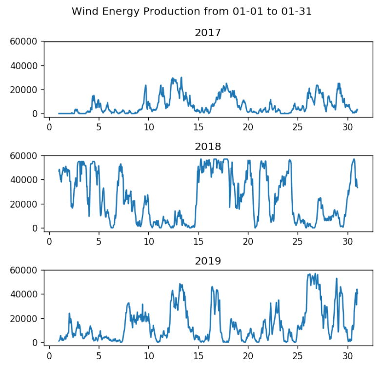
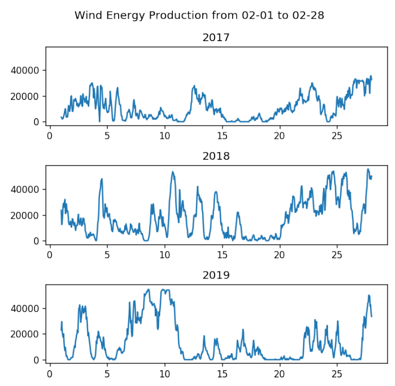
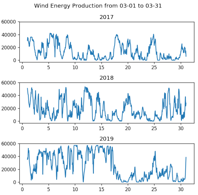
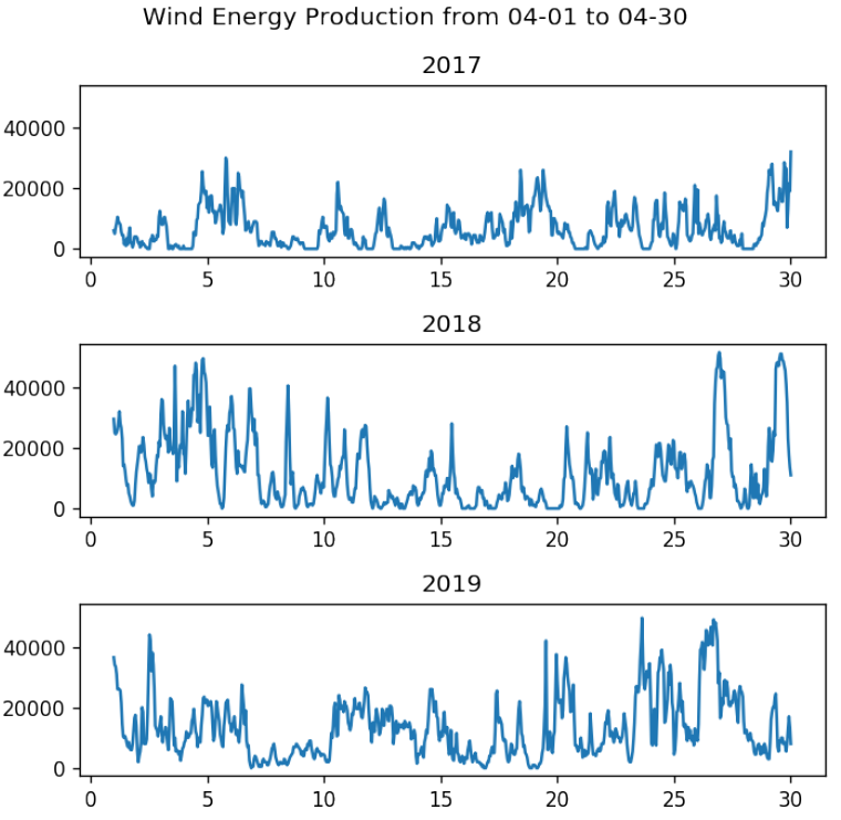
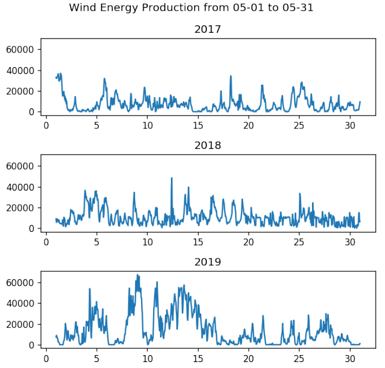
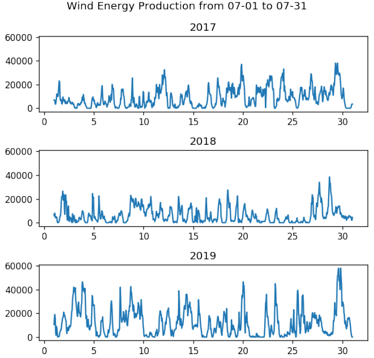
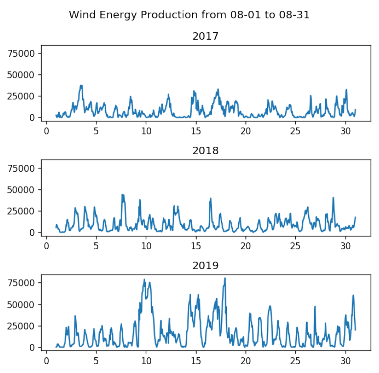
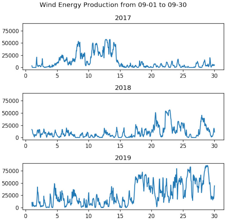
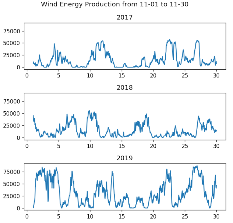
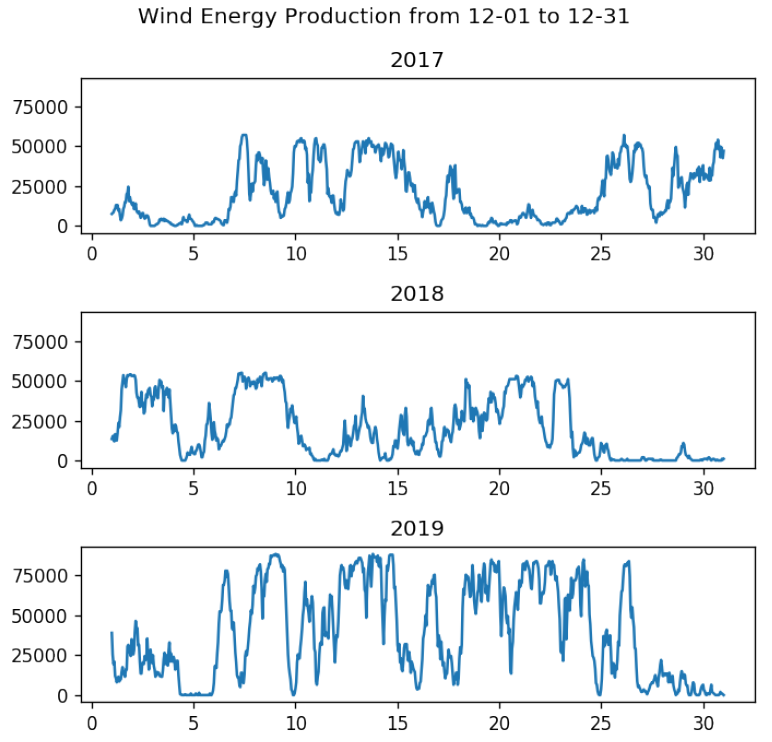
For the purpose of understanding the underlying trends in the raw data sets better, we decided to conduct an in-depth exploratory data analysis. As part of this analysis; we plotted the daily, monthly, quarterly and annual results for the total wind production in 2017, 2018 and 2019 respectively. Furthermore, in order to elaborate, we have also provided a brief set of observations which highlight some of the crucial trends emerging from the respective plots in order to enhance the scope of this preliminary research.

為了更好地理解原始數據集中的潛在趨勢，我們決定進行深入的探索性數據分析。 作為此分析的一部分； 我們分別繪制了2017年，2018年和2019年風電總產量的每日，每月，季度和年度結果。 此外，為了詳細說明，我們還提供了一組簡短的意見，以突出各個地塊中出現的一些關鍵趨勢，以擴大此初步研究的范圍。

Annual Trend:

年度趨勢：

As can be seen from the graph, the wind energy produced has increased in each successive year from 2017 to 2019. The rate of growth has increased over time, with the jump in 2018 to 2019 being greater than the increase in 2017 to 2018.

從圖表中可以看出，從2017年到2019年，風能發電量逐年增加。增長率隨著時間的推移而增加，2018年至2019年的躍升大于2017年至2018年的增長。

Monthly Trend: Energy Production at the monthly level for 2018, followed a classic V-shaped recovery — tipping the least in the month of July. The aggregate levels of energy production were higher in the second half of the year as compared to the first half.

月度趨勢： 2018年的月度能源生產量呈典型的V形回升-在7月份最低。 與下半年相比，下半年能源生產的總水平更高。

Contrarily, Energy Production at the monthly level for both 2017 and 2019 followed a ‘Nike’ swoosh recovery commencing March. For the first two months, the production levels were relatively low. For both of these years, the minimum amount of energy was produced in the summer months, commencing May/ June. Thereafter, the production levels surged in the Autumn months and made their respective highs in the month of December.

相反，2017年和2019年的月度能源生產跟隨著從3月份開始的“耐克”狂風復蘇。 前兩個月的生產水平相對較低。 從這兩個年份開始，從5月/ 6月開始，夏季都產生了最小的能量。 此后，秋季的產量猛增，并在12月達到了各自的最高水平。

Daily Trend: While the day-to-day changes in production remained heavily volatile across all three years, one definite trend that was observed were the increasing volumes of energy production daily on an aggregate level between 2017–2019.

每日趨勢：盡管在過去三年中，每日的生產變化仍然劇烈波動，但可以觀察到的一個明確趨勢是，2017-2019年期間每日的能源生產總量不斷增加。

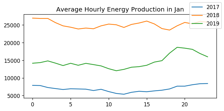
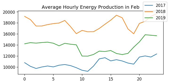
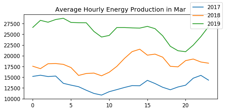
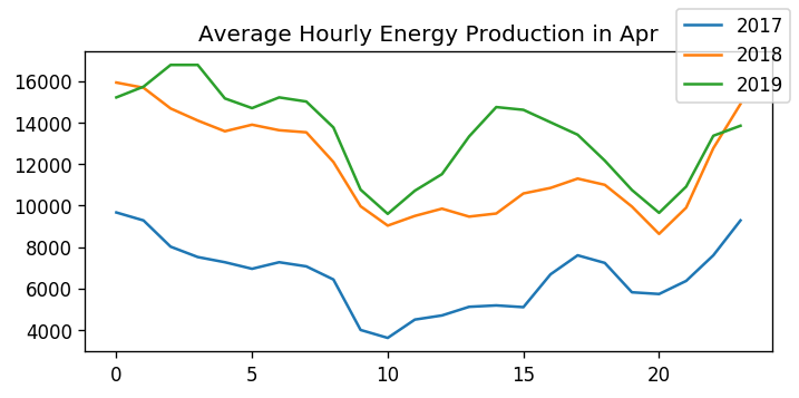
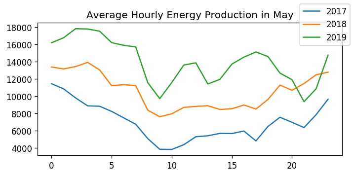
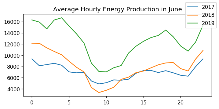
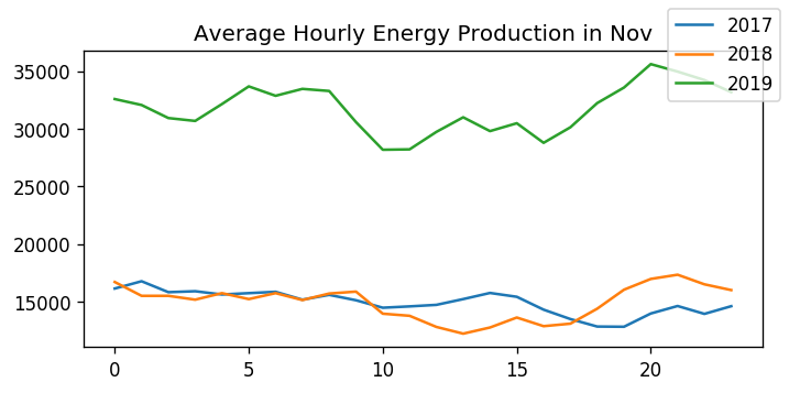
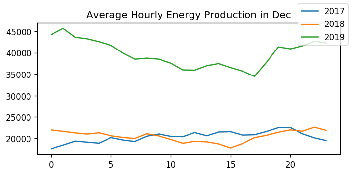
Average Hourly Trend: On plotting the average hourly energy production value in a month wise manner for all three years, we observe that there is a clear seasonal trend as the curves have nearly identical peaks and troughs. There is a clear increase in the magnitude of production every subsequent year, which can be attributed to the increase in wind energy farms in the region.

平均每小時趨勢：在繪制所有三年的每月平均每小時能源生產值時，我們觀察到明顯的季節性趨勢，因為曲線具有幾乎相同的高峰和低谷。 隨后的每一年產量都明顯增加，這可以歸因于該地區風力發電場的增加。

數據準備 (DATA Preparation)

1. Speed/Direction Correlation with Energy Production

   速度/方向與能量產生的關系

We used linear interpolation for the wind speed and direction data to get standardised hourly data. We calculated the Pearson correlation of each feature with the label and found that the wind speed energy was highly correlated to the power output with the correlation coefficient being 0.8. On the other hand, the correlation between wind direction and the label was significantly low with an average value of 0.1 . However, as Pearson correlation method could be misleading when two features are not linearly correlated, we decided to calculate the distance correlation between wind direction and wind energy production since it measured both linear and nonlinear correlation. It was shown that wind direction did not correlate well with power output, The coefficient of approximately 0.2 out of 1 being very low still couldn’t be completely neglected.

我們對風速和風向數據使用了線性插值，以獲得標準化的小時數據。 我們用標簽計算了每個特征的皮爾遜相關性，發現風速能量與功率輸出高度相關，相關系數為0.8 。 另一方面，風向與標簽之間的相關性非常低，平均值為0.1 。 但是，由于當兩個特征不線性相關時，Pearson相關方法可能會產生誤導，因此我們決定計算風向與風能產量之間的距離相關性，因為它同時測量了線性和非線性相關性。 結果表明，風向與功率輸出沒有很好的相關性，仍然無法完全忽略約0.2 / 1的系數非常低。

1. Normalisation (Min-Max v/s Gaussian)

   歸一化(Min-Max v / s Gaussian)

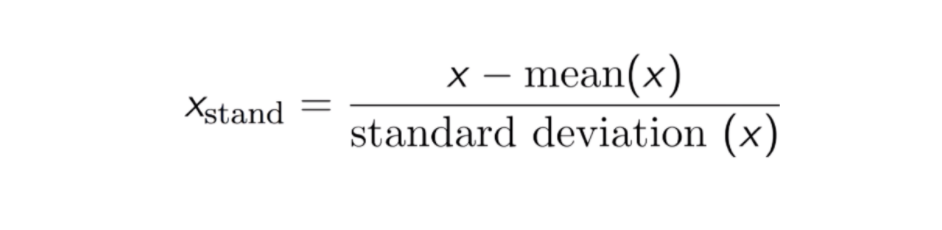
It is imperative for any prediction model to have normalised data as inputs. On plotting our data using histograms, we observed that both energy production values and the wind speed values were following a bell shaped curve. Hence, we decided to normalise the data by subtracting the mean from the values and further dividing it by standard deviation.

任何預測模型都必須將規范化數據作為輸入。 在使用直方圖繪制數據時，我們觀察到能量產生值和風速值都遵循鐘形曲線。 因此，我們決定通過從值中減去平均值并進一步除以標準差來對數據進行歸一化。

We further divided our data by a factor of 2. This allowed us to reduce the range and attain more condensed values, thereby enabling a better learning curve. Furthermore, since the data provided for direction did not follow a bell shaped curve, we simply decided to convert it into radians for ease of calculations in terms of sine and cosine, which also assisted us in reducing the range.

我們將數據進一步除以2 。 這使我們能夠縮小范圍并獲得更多的精簡值，從而獲得更好的學習曲線。 此外，由于提供的方向數據未遵循鐘形曲線，因此我們僅決定將其轉換為弧度，以便于根據正弦和余弦進行計算，這也有助于我們縮小范圍。

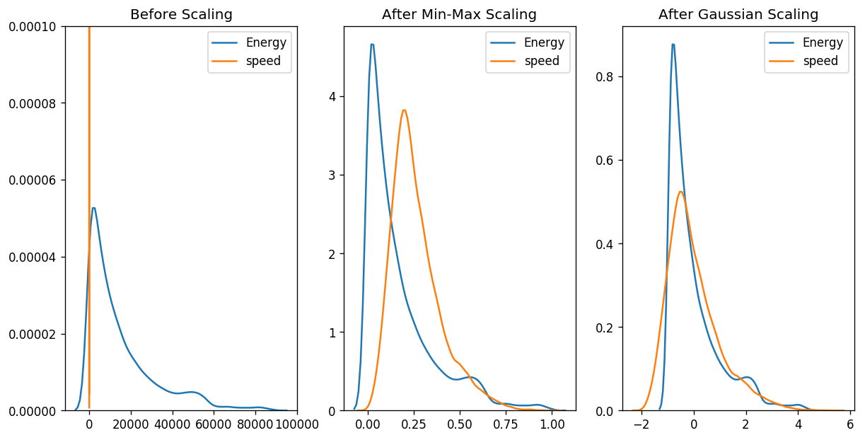
The above figure comparing Min-Max Scaling with Gaussian Scaling.

上圖比較了最小-最大縮放比例和高斯縮放比例。

Issues with Data:

數據問題：

1. Missing historical data in wind/direction:

   缺少風向的歷史數據：

We were using two different models for measuring the wind speed and direction data which were using two different methods to calculate the values. Since, the correlation of the wind speeds/directions with the energy produced as well as the raw values were nearly identical in both models for each of the eight locations (see figure below), we decided to fuse the two and merge the dataset by taking an average of the wind speeds. All values which were either missing or 0 were ignored in the calculations.

我們使用兩種不同的模型來測量風速和風向數據，分別使用兩種不同的方法來計算值。 由于兩個模型中八個位置中的每個位置的風速/風向與產生的能量以及原始值的相關性幾乎相同(請參見下圖)，因此我們決定將兩者融合并合并平均風速。 在計算中將忽略所有丟失或為0的值。

2. Interpolation of direction data:

2.方向數據的插值：

Interpolating direction data was a major challenge that we faced in our model. The primary reason behind this was the fact that direction, contrary to wind speed, is a circular statistic. Instead of converting the data to a standardised variable, we have used raw data for wind direction, by converting them to radians. Although there were methods to standardise the data, we chose not to. This is because of the low correlation of wind direction with energy production. Consequently, we did not use wind direction extensively in our model’s feature engineering.

插值方向數據是我們在模型中面臨的主要挑戰。 其背后的主要原因是，與風速相反的方向是一個循環統計量。 我們沒有將數據轉換為標準變量，而是通過將原始數據轉換為弧度來使用風向。 盡管有使數據標準化的方法，但我們選擇不這樣做。 這是因為風向與能源生產之間的相關性較低。 因此，我們沒有在模型的特征工程中廣泛使用風向。

3. Handling delay of Real Time data of energy production:

3.能源生產實時數據的處理延遲：

In the deployment phase, we used 30 days of past data and 19 hours of forecast data (wind speed and direction) for our features and to handle the delay in the energy production data we used the default 72 hours “previous” interpolation (which gives the previous value during the gap, i.e., the last data point that comes before the desired timestamp in a 72 hour window).

在部署階段，我們將30天的過去數據和19小時的預測數據(風速和風向)用于我們的功能，并且為了處理能源生產數據中的延遲，我們使用了默認的72小時“先前”插值法(間隔期間的前一個值，即72小時窗口中所需時間戳之前的最后一個數據點)。

特征工程 (Feature Engineering)

One should always remember to keep in mind the ‘curse of dimensionality’ while using neural networks in order to avoid faulty analysis. Consequently, it is essential to select the correct amount of features, before advancing to the modelling stage. It is therefore of paramount importance for us to select a certain number of features to use.

人們應該永遠記住在使用神經網絡時要牢記“維數的詛咒”，以避免錯誤的分析。 因此，在進入建模階段之前，必須選擇正確數量的特征。 因此，對于我們而言，選擇要使用的某些功能至關重要。

Firstly, we decided that past data of wind energy production and wind speed, as indicated by the high correlation with our target, would be the two most important features to predict future wind energy production. An increase in speed led to a direct increase in the production values. Due to which we focused more on feature tweaking of Energy Production data and Wind speed data.

首先，我們認為，與目標高度相關的過去的風能發電和風速數據將是預測未來風能發電的兩個最重要的特征。 速度的提高導致生產價值的直接增加。 因此，我們將重點更多地放在了能源生產數據和風速數據的功能調整上。

Secondly, we decided that we should not exclude wind direction data from the neural network since both wind speed and direction affect power output. However, due to the low correlation between wind direction and wind energy production, the inputs of this feature used to train the network were limited solely to future wind forecast as we do not want to put much emphasis on this feature.

其次，我們決定不應該從神經網絡中排除風向數據，因為風速和風向都會影響功率輸出。 但是，由于風向與風能產量之間的相關性較低，因此用于訓練網絡的此功能的輸入僅限于未來的風能預測，因為我們不想過多地強調此功能。

Thirdly, we noticed a nonlinear relationship between wind speed and wind direction, thus using the product of wind speed and wind direction as a feature. Instead of higher orders of wind forecast data, cross-product of speed and direction data offered an easier approach for the neural network to learn the nonlinearity of weather data.

第三，我們注意到風速與風向之間存在非線性關系，因此將風速與風向的乘積作為特征。 代替高階的天氣預報數據，速度和方向數據的叉積為神經網絡提供了一種更簡單的方法來學習天氣數據的非線性。

Finally, on conducting exploratory data analysis we came to the realisation that the Energy Production values and the wind speed had a seasonal trend and our primary aim was to capture this trend for more accurate predictions. Our data window was from the 30 days of past data to 19 days of forecast data giving our model only the necessary features and data requires to capture seasonal trends.

最后，在進行探索性數據分析時，我們意識到能源生產值和風速具有季節性趨勢，而我們的主要目標是捕捉這種趨勢以進行更準確的預測。 我們的數據窗口是從過去30天到19天的預測數據，這為我們的模型提供了捕獲季節性趨勢所需的必要特征和數據。

Difference Network

差異網絡

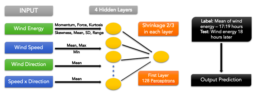
Our neural network was a differencing model, of which the output is added to the average of wind energy data of T-0, T-1 to T-12 to make a prediction of 18 hours in advance. We decided to take the mean from T-0 to T-12 in order to reduce the “noise” of the dataset. Furthermore, we used Smojo programming language for modelling. The list of features is shown as follows:

我們的神經網絡是一個差分模型，該模型的輸出被添加到T-0，T-1至T-12的風能數據的平均值中，從而可以提前18小時進行預測。 我們決定采用T-0到T-12的平均值，以減少數據集的“噪音”。 此外，我們使用Smojo編程語言進行建模。 功能列表如下所示：

我們提供給網絡的詳細輸入如下： (Detailed inputs that we feed to our network are listed as follows:)

: transform

： 轉變

A:19:17 MEAN \ training labels, average for noise removal

A：19：17 MEAN \培訓標簽，用于去除噪音的平均值

A:18 \ testing labels

A：18 \測試標簽

A:0:-12 MEAN \ y0, average for noise removal

A：0：-12 MEAN \ y0，去除噪音的平均值

\ — — — — FEATURES — — — -

\ - - - - 特征 - - - -

A:0:-30 24 momentum \ wind energy, T-0 — T-24, T-1 — T-25,…, T-6 — T-30

A：0：-30 24動量\風能，T-0-T-24，T-1-T-25，…，T-6-T-30

A:0:-30 24 force \ wind energy, 2nd order of 24 DIFFERENCE

A：0：-30 24力\風能，24階二階

A:0:-24 SKEWNESS \ wind energy — skewness

A：0：-24偏斜\風能–偏斜

A:0:-24 KURTOSIS \ wind energy — kurtosis

A：0：-24 KURTOSIS \風能-峰度

A:0:-24 MEAN \ wind energy — mean

A：0：-24平均值\風能-均值

A:0:-24 SD \ wind energy — standard deviation

A：0：-24 SD \風能-標準差

A:0:-24 RANGE \ wind energy — range

A：0：-24范圍\風能-范圍

A:0:-719 MEAN \ wind energy — mean, past 30 days

A：0：-719平均值\風能-過去30天的平均值

A:0:-719 SD \ wind energy — standard deviation, past 30 days

A：0：-719 SD \風能-標準偏差，過去30天

A:0:-719 RANGE \ wind energy — range, past 30 days

A：0：-719 RANGE \風能-范圍，過去30天

A:0:-24 \ wind energy

A：0：-24 \風能

B:19:17 MEAN \ forecasted wind speed — mean

B：19：17 MEAN \預測風速-均值

B:18 \ forecasted wind speed

B：18 \預測風速

B:0:-24 MAX \ past wind speed — max

B：0：-24 MAX \過去的風速-最大

B:0:-24 MIN \ past wind speed — min

B：0：-24 MIN \過去的風速—分鐘

B:-5:-7 MEAN \ past wind speed — mean

B：-5：-7平均值\過去的風速-均值

C:19:17 MEAN \ forecasted wind direction — mean

C：19：17 MEAN \預測風向-均值

C:18 \ forecasted wind direction

C：18 \預測風向

D:19:17 MEAN \ product of forecasted speed and direction

D：19：17 MEAN \預測速度和方向的乘積

D:18 \ product of forecasted speed and direction

D：18 \預測速度和方向的乘積

訓練與預測 (Training and Prediction)

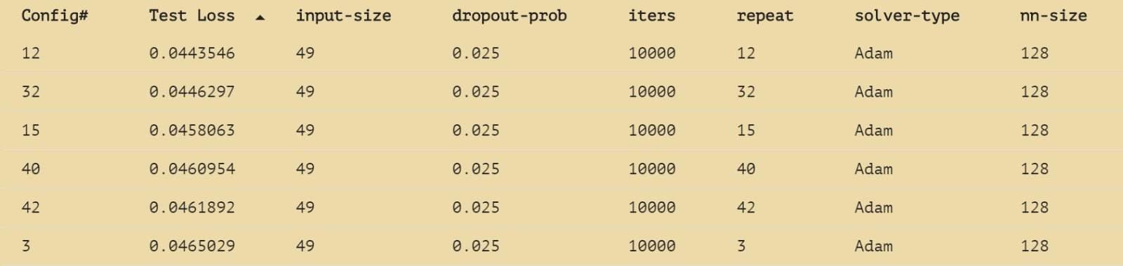
For the training and prediction we tried myriad different configurations, network architectures, dimensionality reduction techniques, scaling methods etc. After over 100 such test cases we obtained our best configuration with the following specifications.

為了進行培訓和預測，我們嘗試了無數種不同的配置，網絡體系結構，降維技術，縮放方法等。經過100多個此類測試案例，我們獲得了具有以下規格的最佳配置。

Deep Learning Neural Network Flowchart

深度學習神經網絡流程圖

The above figure represents the architecture of our neural network prediction model including the datasets and the important statistics fed.

上圖代表了我們的神經網絡預測模型的體系結構，其中包括數據集和重要的統計數據。

Neural Network Specifications

神經網絡規范

After hyperparameter tuning we observed that a neural network of 4 layers followed by a Linear Combinator (LC) gives the most accurate predictions. A deep network with more layers led to overfitting and memorisation of the training samples whereas a really shallow network didn’t fit the actual data so well. On researching and consulting with our trainers we found that the optimum layer-by-layer shrinking factor was around ? and the neural network size / number of perceptrons in the first layer was 128.

經過超參數調整后，我們觀察到4層神經網絡以及線性組合器(LC)給出了最準確的預測。 多層的深層網絡導致訓練樣本的過度擬合和記憶化，而真正淺層的網絡則無法很好地擬合實際數據。 通過與我們的培訓師進行研究和咨詢，我們發現最佳的逐層收縮因子約為1/3，并且第一層的神經網絡大小/感知器數量為128。

Test Loss

測試損失

The persistence loss to be beaten was 0.11117 and the best tost loss obtained after repeated training and configuration tweaking is 0.0443546 .

被擊敗的持久性損失為0.11117 ，經過反復訓練和構形調整后的最佳面包損失為0.0443546 。

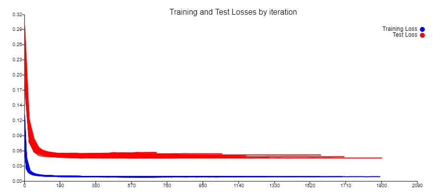
As seen from the figure and the configurations result tables, we beat the persistence result by a relative margin of 60.1 % . Furthermore, we were also able to marginally reduce the test loss to approximately 0.040. However, it induced comparatively more outliers and an additional lag.

從該圖和配置結果表可以看出，我們以60.1％的相對余量擊敗了持久性結果。 此外，我們還能夠將測試損失略微降低至約0.040。 但是，它引起了更多的異常值和額外的滯后。

Predictions:

預測：

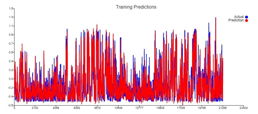
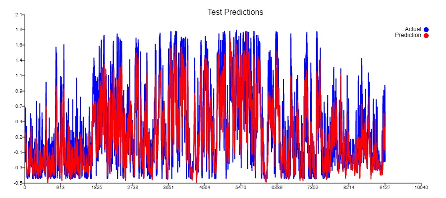
We plotted graphs for Actual vs. Training Prediction, Action vs Testing Prediction and a Lag Correlation graph between Training and Testing phase to visually validate our results.

我們繪制了實際與訓練預測，動作與測試預測的圖表以及訓練與測試階段之間的滯后相關圖，以直觀地驗證我們的結果。

As seen from Fig X. the training predictions mostly fit the actual data leading to finer training. However, the test predictions on the other hand rigidly followed the peaks and valleys of the actual data, thereby leading in slightly under-predicting.

從圖X可以看出，訓練預測大多適合實際數據，從而可以進行更精細的訓練。 但是，另一方面，測試預測嚴格遵循實際數據的峰值和谷值，從而導致預測不足。

We further plotted scatter plots to check the distribution of our best configuration and observe the nature of all prevalent outliers

我們進一步繪制了散點圖，以檢查最佳配置的分布并觀察所有流行異常值的性質

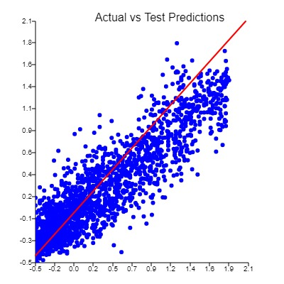
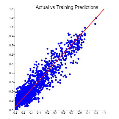
As seen from the above figures, while on the one hand, the Actual vs Training Predictions plot is roughly a straight line with very few outliers, on the other the Actual vs Testing Predictions Plot had a majority of points — either really near to the red line or below it. This was an indication of the fact that our model was under-predicting more than it was over predicting.

從以上數據可以看出，一方面，實際與訓練預測圖之間的直線大致是很少的異常值；另一方面，實際與測試預測圖之間的關系主要是點–要么實際上接近紅色線或下方。 這表明我們的模型對預測的誤解多于對預測的誤解。

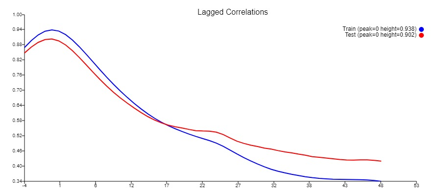
The Lagged Correlation Graph depicted that both the Training and the Testing curve had a zero lag peak with almost similar heights. This was an indication of the fact that there was no expedition or delay in our predictions ultimately leading to more accurate results.

滯后相關圖描述了訓練曲線和測試曲線都具有零延遲峰，高度幾乎相似。 這表明以下事實：我們的預測沒有任何探索或延遲，最終會導致更準確的結果。

Judgement Calls made based on Problem Specification

根據問題說明進行判斷調用

The trading algorithm defined for wind energy trading penalises over-prediction more than under-prediction with a ratio of 2:1. Due to this reason, we tweaked our model in such a manner that over-prediction is more harshly penalised. This can also be seen from the Actual vs Test Prediction Line Graph and Scatter Plot. Our total profit improved by approximately 23 % on adopting this strategy.

為風能交易定義的交易算法會以2：1的比率對高估多于低估進行懲罰。 由于這個原因，我們對模型進行了調整，以至于過高的預測更為嚴厲。 這也可以從實際與測試預測線圖和散點圖看出。 采用這一策略，我們的總利潤提高了約23％ 。

Since our goal was to maximise profit, we took the decision to pursue a fine balance between the test loss and the lagged correlation curve. A lower loss, was in most cases leading to a worse correlation curve. We prioritised the lagged correlation curve over reducing test loss as the trading algorithm is very volatile and due to its high sensitivity, even a minor lag would significantly change the profit for worse.

由于我們的目標是使利潤最大化，因此我們決定在測試損失和滯后的相關曲線之間尋求良好的平衡。 較低的損耗在大多數情況下會導致較差的相關曲線。 由于交易算法非常不穩定，并且由于其高靈敏度，我們優先考慮滯后相關曲線，以降低測試損失，即使是很小的滯后也會嚴重改變利潤。

局限性 (Limitations)

Our model tends to under-predict by a large margin during high energy production phases (especially above 35 kWh). Additionally, it sometimes fails to efficiently capture a downward trend, possibly due to lag in the predictions. These might be because of the low production capacity pattern in 2017 that the model learns that affects the predictions during high production phase.

在高能發電階段(尤其是35 kWh以上)，我們的模型往往會出現較大幅度的預測不足。 另外，有時由于預測的滯后，有時無法有效捕獲下降趨勢。 這可能是由于該模型了解到的2017年低產能模式會影響高產能階段的預測。

To tackle these limitations, we think of implementing a loss function using weighted mean squared error that puts more weight on the squared error of energy data of higher values. Another approach is to exclude data in 2017 and use a loss function that penalises over-prediction more.

為了解決這些局限性，我們考慮使用加權均方誤差來實現損失函數，該函數將更大的權重放在較高值的能量數據的平方誤差上。 另一種方法是在2017年排除數據，并使用損失函數來懲罰過度預測。

結論與教訓 (Conclusion and Lessons)

To conclude with, we would like to highlight all of the crucial steps that we took as well as the major lessons that we learnt while analysing, processing, training and testing the data. The first step we undertook was to conduct the exploratory data analysis for the purpose of understanding the underlying trends in the data and subsequently plot the frequency distributions of the raw data in order to decide which normalisation to use. Among some of the most important observations made, were the facts that as per the annual trend plotted, energy produced in every successive year was increasing over time and as per the quarterly and daily trends produced, the levels of volatility and volume produced of energy were far greater in 2018 and 2019 as compared to 2017.

最后，我們要重點介紹我們在分析，處理，訓練和測試數據時所采取的所有關鍵步驟以及所學的主要課程。 我們進行的第一步是進行探索性數據分析，以了解數據的潛在趨勢，然后繪制原始數據的頻率分布，以決定使用哪種歸一化方法。 在一些最重要的觀察結果中，有一個事實是，按照年度趨勢繪制，每隔一年的能源產量隨著時間的推移而增加，并且按照產生的季度和每日趨勢，能源的波動水平和發電量與2017年相比，2018年和2019年的數字要大得多。

Next, we used linear interpolation for the wind speed and the wind direction data to get the standardised hourly data. As per our findings, we found a high correlation between wind speed and the power output but a relatively lower correlation between wind direction and power output. However, provided that we were using the Pearson correlation method which could be misleading in case of non-linear correlation between two features — we decided to calculate the distance correlation between wind direction and wind energy production. Having done so, we eventually concluded that although there wasn’t a strong correlation between wind direction and power output, we still couldn’t totally neglect the feature due the presence of a minimalistic correlation.

接下來，我們對風速和風向數據使用線性插值，以獲得標準化的小時數據。 根據我們的發現，我們發現風速與功率輸出之間的相關性較高，而風向與功率輸出之間的相關性相對較低。 但是，假設我們使用的Pearson相關方法在兩個要素之間存在非線性相關的情況下可能會產生誤導，因此我們決定計算風向與風能產量之間的距離相關性。 這樣做之后，我們最終得出結論，盡管風向與功率輸出之間沒有很強的相關性，但是由于存在極簡相關性，我們仍然不能完全忽略該特征。

After this we decided on the best technique to normalise our data. Having plotted the data using histograms, we observed that both energy production values and the wind speed values were following a bell shaped curve because of which we decided to subtract the values by the mean and divide it further by the SD. We further divided these values by 2 to condense the range. As for the data on direction, we simply decided to convert into radians for the ease of calculation. However, it must be highlighted that we did face some issues with the data such as the presence of missing historical data, dealing with interpolating the direction data and handling the delay of real time data for energy production.

之后，我們決定采用最佳技術對數據進行標準化。 使用直方圖繪制數據后，我們觀察到能量產生值和風速值均遵循鐘形曲線，因此我們決定將這些值除以平均值，再除以SD。 我們進一步將這些值除以2以壓縮范圍。 至于方向數據，為了簡化計算，我們只是決定將其轉換為弧度。 但是，必須強調的是，我們確實在數據方面遇到了一些問題，例如缺少歷史數據，處理方向數據的插值以及處理用于發電的實時數據的延遲。

Our extensive data analysis helped us with the feature engineering and we were able to select useful features rather early in the process. Apart from the wind energy production, wind speed and wind direction data, to handle the non-linear relationship between the wind speed and direction, we used the product of the two as a feature as well. Furthermore, our neural network was based in a differencing model with the mean from T-0 to T-12 taken to reduce the noise of the dataset. During the training and prediction phase we tried a variety of configurations and dimensionality reduction techniques to conclude that a neural network of 4 layers followed by a Linear combinator was giving us the most accurate predictions. Also we concluded that the optimum layer-by-layer shrinking factor was around ? and the neural network size / number of perceptrons in the first layer was 128. Having used all of the aforementioned specifications we finally arrived at the point where our best configuration beat persistence result by a relative margin of 60.1%.

我們廣泛的數據分析幫助我們進行了功能設計，并且能夠在此過程的早期選擇有用的功能。 除了產生風能，風速和風向數據以外，為了處理風速和風向之間的非線性關系，我們還使用兩者的乘積作為特征。 此外，我們的神經網絡基于差分模型，取平均值從T-0到T-12以減少數據集的噪聲。 在訓練和預測階段，我們嘗試了多種配置和降維技術，得出的結論是，四層神經網絡后接線性組合器，為我們提供了最準確的預測。 我們還得出結論，最佳的逐層收縮因子約為1/3，第一層的神經網絡大小/感知器數為128。使用所有上述規范，我們終于到達了最佳配置的地步持久性的相對幅度為60.1％。

Lastly, having plotted the graphs for Actual vs. Training Prediction, Action vs Testing Prediction and the Lag Correlation, we observed that in case of the test predictions, our model was rigidly following the peaks and valleys of the actual data, thereby slightly under-predicting. This observation was also consistent with the results observed from the Actual vs Training Prediction scatter plot graph.

最后，在繪制了實際預測與訓練預測，動作預測與測試預測以及滯后相關性的圖表后，我們觀察到在進行測試預測的情況下，我們的模型嚴格遵循實際數據的波峰和波谷，因此略低于-預測。 該觀察結果也與從“實際與訓練預測”散布圖圖中觀察到的結果一致。

— — X— — — — — —X — — — — — — — — —X — — — — — — — — X — —

— — X — — — — — — — X — — — — — — — — — X — — — — — — — — — — — — X –