Simple OLS Regression, Pairs Bootstrap Resampling, and Hypothesis Testing to observe the effect of Hubble’s Law in Python.

通過簡單的OLS回歸，配對Bootstrap重采樣和假設檢驗來觀察哈勃定律在Python中的效果。

In this post, we will revisit Hubble’s Law and examine the original dataset he used by running an Ordinary Least Squares Linear Regression on the 24 measurements of distances and recessional velocities of extra-galactic nebulae. Then, we will use a pairs bootstrap resampling to calculate the RSS Minima and perform a hypothesis test on the measured effect of galactic distance on recessional velocities.

在本文中，我們將回顧哈勃定律，并通過對銀河外星云的距離和后退速度的24個測量值進行普通最小二乘線性回歸來檢驗他使用的原始數據集。 然后，我們將使用成對的自舉重采樣來計算RSS最小值，并對銀河距離對后退速度的測量影響進行假設檢驗。

Based on the results of the hypothesis test we can conclude with a high degree of statistical signficance that distance has an observed effect on the recessional velocity of galaxies. This is concrete evidence of Hubble’s Law that the universe is constantly expanding.

根據假設檢驗的結果，我們可以得出高度的統計意義，即距離對星系的后退速度有明顯影響。 這是哈勃定律證明宇宙不斷膨脹的具體證據。

Before we get into that let’s familiarize ourselves with Hubble’s Law.

在開始討論之前，讓我們熟悉哈勃定律。

哈勃定律 (Hubble’s Law)

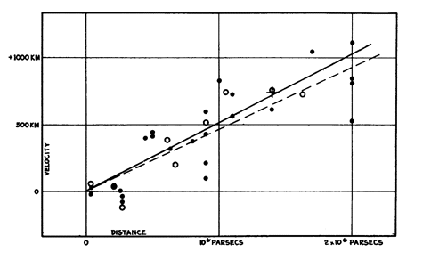
In Edwin Hubble’s famous PNAS article “A relation between distance and radial velocity among extra-galactic nebulae” (1), Hubble provided evidence for one of science’s greatest discoveries: the expanding universe. Hubble demonstrated that galaxies are moving away from Earth with a recession velocity that is correlated to their distance from Earth. In other words, galaxies that are further away from Earth move away faster than nearby galaxies. This is commonly referred to as Hubble’s Law. Hubble’s classic graph of observed velocity vs. distance for nearby galaxies (presented above) visualizes this phenomenon. This graph has become a milestone in the scientific community, as it displays the linear relationship between galactic recessional velocity (v) and distance from Earth (d):

在埃德溫·哈勃(Edwin Hubble)著名的PNAS文章“銀河外星云之間的距離與徑向速度之間的關系”(1)中，哈勃為科學上最偉大的發現之一：膨脹中的宇宙提供了證據。 哈勃證明，星系正在以與地球到地球的距離相關的衰退速度離開地球。 換句話說，距離地球較遠的星系比附近的星系移動得更快。 這通常稱為哈勃定律。 哈勃(Hubble)關于附近星系觀測到的速度與距離的經典關系圖(如上所示)將這一現象形象化。 這張圖已成為科學界的里程碑，因為它顯示了銀河退縮速度(v)與距地球的距離(d)之間的線性關系：

v = Ho x d

v = Ho xd

Here v is the galaxy’s recessional velocity and d is the galaxy’s distance from Earth. Ho is an empirically determined constant called Hubble’s constant. Even though the expansion rate is persistent in all directions at any given time, it changes throughout the lifetime of the universe. The well-calibrated expansion rate at the present time, Ho, is about 70 kilometers per second per megaparsec (note on units used here: recession velocity is in kilometers per second and distance is in megaparsec, 1 megaparsec = 1M parsecs, 1 parsec = 3.26 light-years). (2)

這里v是星系的后退速度， d是星系到地球的距離。 Ho是根據經驗確定的常數，稱為哈勃常數。 即使在任何給定時間在所有方向上都具有持久的膨脹率，它在整個宇宙的生命周期中都會發生變化。 目前，經過良好校準的擴展速度Ho約為每秒每兆帕秒70公里(此處使用的單位請注意：后退速度以千米每秒為單位，距離以兆帕秒為單位，1兆帕秒= 1M帕秒，1帕秒= 3.26光年。 (2)

Hubble’s remarkable feat was obtained using a very small sample of measurements of velocities and distances for 24 nearby galaxies. The distances to these galaxies were inaccurately measured from the visible brightness of their stars. In addition to plotting all of the individual 24 galaxies in the diagram, Hubble also grouped them into 9 clusters (open circles on Hubble’s diagram) based on their closeness in direction and distance, as a means of minimizing the scatter. Hubble’s experiment was conclusive in convincing the scientific community of the existence of the expanding universe. (2)

哈勃的非凡成就是使用非常小的24個附近星系的速度和距離測量樣本獲得的。 距這些星系的距離是根據其恒星的可見亮度進行的不準確測量。 除了在圖中繪制所有24個星系之外，哈勃還根據方向和距離的緊密程度將它們分為9個簇(哈勃圖上的空心圓)，以最大程度地減少散射。 哈勃的實驗在說服科學界相信不斷膨脹的宇宙的存在方面是結論性的。 (2)

Hubble’s diagram shows a strong linear relationship between velocity and distance. What makes this graph profound is the extensive implications of the observed trend: we live in a large, dynamically evolving universe that is expanding all directions. It is not the type of universe that Albert Einstein assumed in 1917. In fact, Einstein factored in a cosmological constant into his equations to keep the universe static, as it was believed to be at the time. Contrary to Einstein’s beliefs, Hubble’s results suggested that the universe has been expanding for billions of years, from an early beginning of the “Big Bang” up until the present. (2)

哈勃圖顯示了速度和距離之間的強線性關系。 使該圖更深刻的是觀察到的趨勢的廣泛含義：我們生活在一個巨大的，動態演化的宇宙中，宇宙在向各個方向擴展。 這不是阿爾伯特·愛因斯坦(Albert Einstein)在1917年所假定的那種宇宙。實際上，愛因斯坦將宇宙學常數納入其方程式中，以保持宇宙的靜態性，這在當時被認為是這樣。 與愛因斯坦的看法相反，哈勃的結果表明，從“大爆炸”的早期開始到現在，宇宙已經膨脹了數十億年。 (2)

Although Hubble successfully displayed the beautiful linear relationship in his diagram, Hubble’s values for his distances in 1929 were too small by a factor of ~7. The expansion rate Ho was also too large by the same factor. However, despite this large imprecision and its great ramifications for the expansion rate and age of the universe, Hubble’s discovery of the expanding universe is not affected. The underlying linear equation of v ～ d still holds true! (2)

盡管哈勃在圖表中成功顯示出漂亮的線性關系，但哈勃在1929年的距離值太小了約7倍。 出于相同的原因，膨脹率Ho也太大。 但是，盡管存在很大的不精確性，并且對宇宙的膨脹率和年齡有很大的影響，但哈勃關于宇宙膨脹的發現并沒有受到影響。 v的基本線性方程?d仍然適用！ (2)

Note that Einstein’s theory of relativity forecasts deviations from a strictly linear interpretation of Hubble’s law. The amount of deviation depends on the total mass of the universe. A greater understanding of Hubble’s law can inform us about the amount of total matter in the universe. It might also provide more information about dark matter… (3)

請注意，愛因斯坦的相對論預測偏離哈勃定律的嚴格線性解釋。 偏差量取決于宇宙的總質量。 對哈勃定律有更深入的了解可以使我們了解宇宙中總物質的數量。 它還可能提供有關暗物質的更多信息……(3)

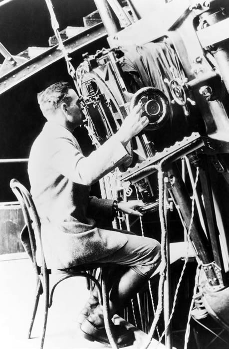
Hubble’s Law was the primary observational evidence in support of the Big Bang theory. Hubble was well renown for his discoveries and in 1990 NASA named the Hubble space telescope after him. (4)

哈勃定律是支持大爆炸理論的主要觀察證據。 哈勃因其發現而享譽世界。1990年，美國國家航空航天局(NASA)以他的名字命名了哈勃太空望遠鏡。 (4)

Excellent! With that out of the way, now we can start diving into all the fun we’re going to have with hacker stats and Ordinary Least Squares (OLS) Regression. Let’s get started.

優秀的！ 有了這種方式，現在我們就可以開始研究黑客統計數據和普通最小二乘(OLS)回歸帶來的所有樂趣。 讓我們開始吧。

實驗設計(方法論) (Experimental Design (Methodology))

• Exploratory Data Analysis (EDA).
  探索性數據分析(EDA)。
• Adjust galactic distances by a factor of 7.
  將銀河距離調整7倍。
• OLS using the original Hubble dataset of 24 measurements of galactic distances and recession velocities.
  OLS使用最初的哈勃數據集，其中包含24個銀河距離和后退速度測量值。
• Pairs Bootstrap Resampling of 24 measurements.
  配對Bootstrap重采樣24個測量值。
• Hypothesis Test → measure the effect of distance on recession velocities.
  假設檢驗→測量距離對衰退速度的影響。

關于數據 (About the Data)

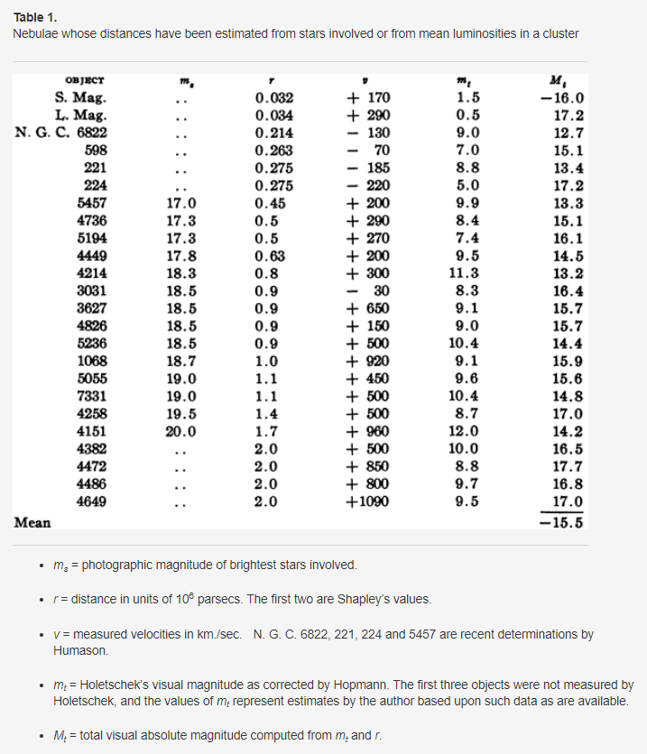
Source: “A relation between distance and radial velocity among extra-galactic nebulae” by Edwin Hubble. (1)

資料來源：埃德溫·哈勃(Edwin Hubble)的“銀河外星云之間的距離與徑向速度之間的關系”。 (1)

• Object Name: Name of the galaxy.

  對象名稱：星系的名稱。

• Distance [Mpc] (r): Distance from Earth in megaparsecs. 1 megaparsec = 1M parsecs, 1 parsec = 3.26 light-years.

  距離[Mpc](r)：距地球的距離，單位為兆帕。 1兆帕秒= 1M帕秒，1帕秒= 3.26光年。

• Velocity [Km/second] (v): Recessional velocity, how fast a galaxy is moving away from Earth. Recessional velocity was recorded in kilometers per second.

  速度[Km / second](v)：衰退速度，銀河系離開地球移動的速度。 衰退速度以公里每秒記錄。

**Note to my technical readers: If you are interested in the Python code that I used to generate the plots, calculations, etc. feel free to check out my GitHub repo.**

**我的技術讀者注意：如果您對我用來生成繪圖，計算等的Python代碼感興趣，請隨時查看我的 GitHub存儲庫 。**

EDA (EDA)

The first thing we will do is look at the normalized deviations of distances and recessional velocities to?examine?their?relationship. The mean describes the center of the data. The standard deviation describes the spread of the data. It is convenient to normalize two variables in order to perform a fair comparison.

我們要做的第一件事是查看距離和后退速度的歸一化偏差，以檢查它們之間的關系。 平均值描述數據的中心。 標準差描述數據的傳播。 標準化兩個變量以便進行公平比較很方便。

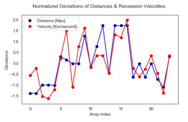
With the exception of the first couple of measurements, upon visual inspection of the two normalized arrays of the deviations the galactic distances and their recession velocities seem to be highly correlated. Let’s adjust the distance values?and?generate?summary?statistics?of?our?data.

除了前幾對測量值以外，在目視檢查兩個標準化的偏差陣列后，銀河距離及其后退速度似乎高度相關。 讓我們調整距離值并生成數據的摘要統計信息。

Adjust Distances by Factor of 7

以7的系數調整距離

Now we are going to adjust the distance values by multiplying them by a factor of 7. We can look at the result of our adjustment through descriptive statistics.

現在，我們將距離值乘以7來調整距離值。我們可以通過描述性統計數據查看調整結果。

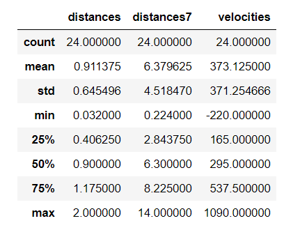
Despite the increase in distance by a large factor of 7, recessional velocity and galactic distance are still highly correlated. Let’s calculate the Pearson correlation coefficient and visualize the correlation with the adjusted distance variable via a scatter plot.

盡管距離增加了7倍，但后退速度和銀河距離仍然高度相關。 讓我們計算皮爾遜相關系數，并通過散點圖可視化與調整后的距離變量的相關性。

Correlation

相關性

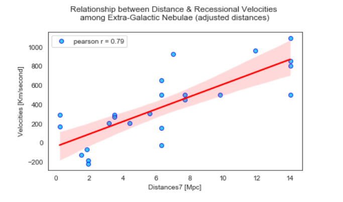
Aside from the adjustment of the x-axis, this graph doesn’t look much different than the one that Hubble created. The data exhibits a strong linear relationship with a Pearson correlation coefficient of ~0.8. Next we will perform an Ordinary Least Squares Regression to further understand this relationship as a result of a linear function.

除了調整x軸外，此圖看起來與哈勃創建的圖沒有太大不同。 數據表現出很強的線性關系，皮爾遜相關系數約為0.8。 接下來，我們將執行普通最小二乘回歸，以進一步了解線性函數的關系。

最小二乘 (OLS)

The regression results below were generated via the statsmodels ols() API in Python.

下面的回歸結果是通過Python中的statsmodels ols()API生成的。

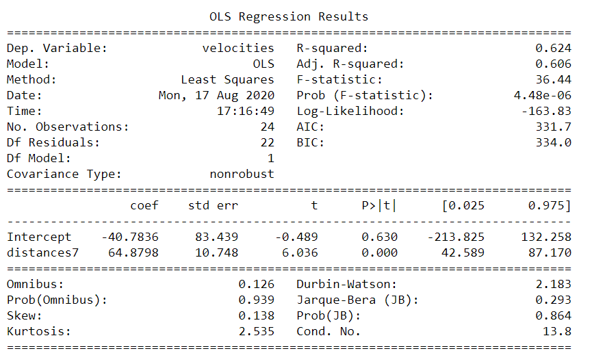
For every unit increase in distance, recessional velocity increases by 64.88 km per second.

每增加單位距離，后退速度將增加64.88 km / s。

According to the R-squared value, 62% of the variance of recession velocities are explained by distances.

根據R平方值，用距離解釋了衰退速度變化的62％。

We’ve already observed Hubble’s Law with a couple of lines of Python code. We examined correlation and concluded with enough confidence that the majority of the variance can be explained by the model. Technically, we could stop at this point and call it day. But let’s take this a step further and understand the residuals like any good scientist would.

我們已經用幾行Python代碼觀察了哈勃定律。 我們檢查了相關性，并以足夠的信心得出結論，該模型可以解釋大部分方差。 從技術上講，我們可以在這一點上停下來并將其命名為“ day”。 但是，讓我們更進一步，像任何優秀科學家一樣理解殘差。

Residuals, RSS and RMSE

殘差，RSS和RMSE

If we interpret R-squared as the variances that can be explained by our OLS model, the residual sum of squares (RSS) represents the amount of errors that are not explained by the model.

如果我們將R平方解釋為可以由我們的OLS模型解釋的方差，則殘差平方和(RSS)表示該模型無法解釋的誤差量。

The solution of OLS regression is the set of coefficient values for which the RSS is minimal. We’ll revisit this topic when we look at bootstrap resampling in the next section.

OLS回歸的解決方案是RSS最小的一組系數值。 在下一節中，我們將在介紹引導程序重采樣時重新討論該主題。

Here we have Root Mean Square Error (RMSE) of ~223, which can be interpreted as the spread of prediction errors, or how concentrated the data is around the line of best fit. Let’s look at a probability plot to visualize the spread of residuals.

在這里，我們的均方根誤差(RMSE)為?223，可以解釋為預測誤差的散布，或者數據在最佳擬合線附近的集中程度。 讓我們看一下概率圖，以可視化殘差的分布。

The probability plot of the residuals of our OLS model is approximately linear, supporting the assumption that the error terms are normally distributed.

我們的OLS模型殘差的概率圖近似線性，支持誤差項呈正態分布的假設。

Again we could also stop right here, but we’re going to keep moving and generate some bootstrap replicates to validate some of the conclusions we’ve witnessed from OLS Regression and uncover a couple of new ones?of?our?own.

同樣，我們也可以在這里停止，但是我們將繼續前進并生成一些引導程序副本，以驗證從OLS Regression見證的一些結論，并發現我們自己的一些新結論。

使用雙自舉重采樣 (Resampling with Pairs Bootstraps)

Pairs bootstrap involves resampling pairs of data with replacement. Each collection of pairs fit with a regression model. We will do this again, and again, and again n number of times generating bootstrap n sample statistics from the explanatory and dependent variables, in addition to model parameter estimates after running the OLS model n number of times. We will also calculate the RSS Minima using Bootstrap Resampling to identify the linear equation that best minimizes the errors.

Pairs bootstrap涉及重新采樣數據對并進行替換。 對的每個集合均符合回歸模型。 我們會再次做到這一點，又一次，又一次次從生成的解釋變量和因變量的自舉n個采樣統計n個，除了模型參數估計運行時間的OLS模型n個后。 我們還將使用Bootstrap重采樣來計算RSS最小值，以識別最能使誤差最小的線性方程。

The goal is to use bootstrap resampling to compute one mean for each sample and create a distribution of sample means and then compute the standard error to quantify the uncertainty in the sample statistic as an estimator for the population average and standard deviation. This comes in very handy since we don’t know the true values for the population average or standard deviation. Instead, we will infer it using bootstrap resampling.

目標是使用自舉重采樣為每個樣本計算一個均值，并創建樣本均值的分布，然后計算標準誤差以量化樣本統計數據中的不確定性，作為總體平均值和標準偏差的估計量。 這非常方便，因為我們不知道總體平均值或標準差的真實值。 相反，我們將使用引導重采樣來推斷它。

According to the central limit theorem, if we generate enough replicates the resampled distributions will follow a normal distribution, which is one of the assumptions for a hypothesis test. More on that in the next section. For now, let’s generate 1,000 paired replicates for each variable.

根據中心極限定理，如果我們生成足夠多的重復項，則重新采樣的分布將遵循正態分布，這是假設檢驗的假設之一。 下一節將對此進行更多介紹。 現在，讓我們為每個變量生成1,000個成對的重復。

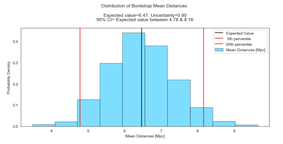
Through way of bootstrap, we inferred that the expected average value of galactic distances is 6.47 Mpc with an uncertainty of about 1 Mpc. This is really close to the sample mean and standard deviation we generated early on. In addition, we can infer with 95% confidence that the true population average lies somewhere between 4.78 and 8.16 Mpc, based on the data provided.

通過自舉，我們推斷銀河距離的預期平均值為6.47 Mpc，不確定性約為1 Mpc。 這確實接近我們早期生成的樣本均值和標準差。 此外，根據提供的數據，我們可以以95％的置信度推斷出真正的人口平均數介于4.78和8.16 Mpc之間。

Notice we have a black line in the middle to mark the expected value. Uncertainty here is just one measure of the spread of the distribution of sample means. Moreover, notice the uncertainty we computed also fits inside the confidence interval. You can think of the uncertainty as the one-sigma confidence interval.

注意，中間有一條黑線標記期望值。 這里的不確定度只是衡量樣本均值分布范圍的一種方法。 此外，請注意，我們計算出的不確定性也適合置信區間內。 您可以將不確定性視為一個1西格瑪的置信區間。

In addition, the vertical red lines mark the 5th (left) and 95th (right) percentiles, which denote the extent of the confidence interval or the range of values containing the inner 95% of sample means.

此外，垂直紅線標記第5個(左)和第95個(右)百分位數，表示置信區間的范圍或包含內部95％樣本均值的值的范圍。

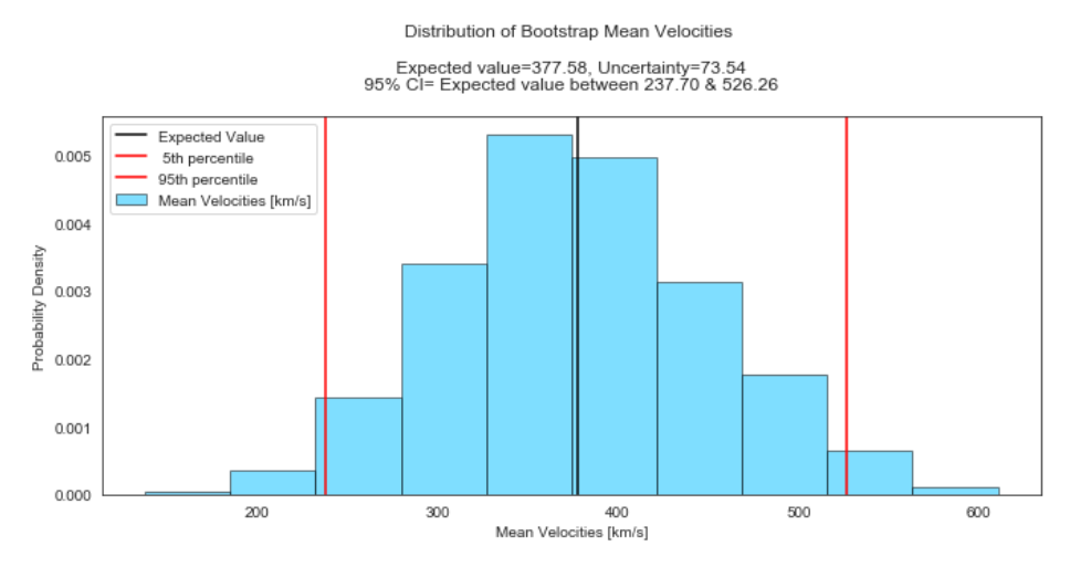
Similarly for velocities, we inferred that the expected average value of velocities is about 378 km per second with an uncertainty of about 74 km per second. In addition, we can infer with 95% confidence that the true population average lies somewhere between 238 and 526 km per second, based on the data provided.

同樣，對于速度，我們推斷速度的期望平均值約為每秒378公里，不確定度約為每秒74公里。 此外，根據提供的數據，我們可以以95％的置信度推斷出真實的平均人口數量在每秒238至526 km之間。

Now we’re going to conduct a similar exercise, this time with the model slope and intercept parameters. That’s right! You can also use bootstrap resampling to compute the estimate, standard error, and confidence interval for OLS model parameters, all thanks to the central limit theorem. We’re basically going to use each pairs bootstrap replicate as an input into an OLS model to generate bootstrap slope and intercept estimates. Let’s give it a try.

現在，我們將使用模型斜率和截距參數進行類似的練習。 那就對了！ 您還可以使用引導重采樣來計算OLS模型參數的估計值，標準誤差和置信區間，這全都歸功于中心極限定理。 基本上，我們將使用每對引導復制作為OLS模型的輸入，以生成引導斜率和截距估計。 試一試吧。

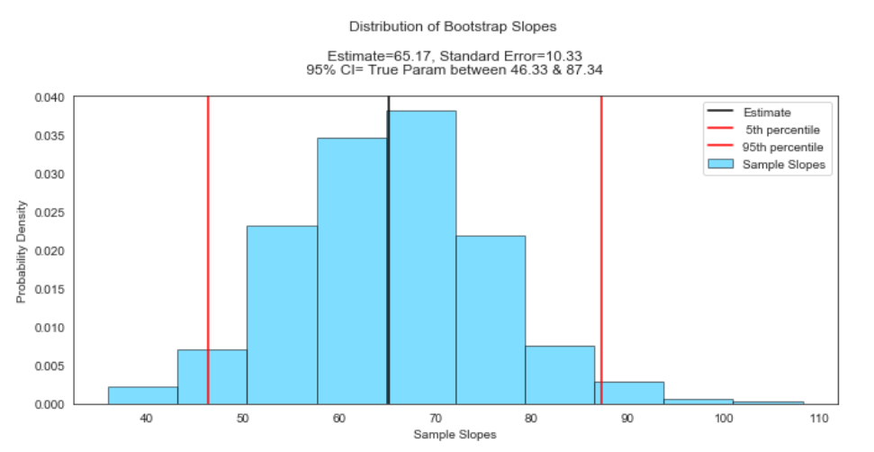
We inferred that the estimate of the slope is 65.17 km per second/Mpc with a standard error of 10.33 km per second/Mpc. We are 95% confident that the true slope lies somewhere between 46.33 and 87.34 km per second/Mpc, based on the data provided.

我們推斷斜率的估計值為65.17 km / s / Mpc，標準誤差為10.33 km / s / Mpc。 根據提供的數據，我們有95％的把握是真實的斜率在46.33和87.34 km /秒/ Mpc之間。

Note that this is very close to the summary output of statsmodels ols().

請注意，這與statsmodels ols()的摘要輸出非常接近。

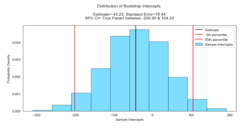
We inferred that the estimate of the intercept is -43.23 km per second with a standard error of 78.44 km per second. We are 95% confident that the true intercept lies somewhere between -200.99 and 104.23 km per second, based on the data provided.

我們推斷，截距的估計值為每秒-43.23 km，標準誤為每秒78.44 km。 根據提供的數據，我們有95％的信心確定真正的截距在每秒-200.99至104.23 km之間。

Now we’re going to generate the RSS Minima via Pairs Bootstrap Resampling.

現在，我們將通過Pairs Bootstrap重采樣來生成RSS最小值。

Visualizing the RSS Minima

可視化RSS最小值

Recall when we looked at RSS before, the solution of OLS is the set of coefficient values for which the RSS is minimal. Now we’re going to use the same replicates we generated to visualize the RSS Minima. Then we’re going to retrieve the model parameters (slope and intercept) that generated the RSS Minima.

回想一下我們以前看過RSS時，OLS的解是RSS最小的一組系數值。 現在，我們將使用生成的相同副本來可視化RSS Minima。 然后，我們將檢索生成RSS最小值的模型參數(坡度和截距)。

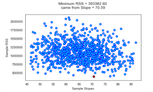
Amazing! The best slope and intercept are the ones out of arrays of slopes and intercepts that yielded the minimum RSS value. Notice that our slope value is almost equivalent to the well-calibrated expansion rate (Ho) at the present time.

驚人！ 最佳斜率和截距是那些產生最小RSS值的斜率和截距數組中的斜率和截距。 請注意，目前我們的斜率值幾乎等于經過良好校準的膨脹率( Ho )。

Behind the scenes, we used the 95% confidence intervals that we generated for the slope and intercept estimates to filter out model parameter values that weren’t within range.

在幕后，我們使用為斜率生成的95％置信區間并截取估計值，以過濾掉不在范圍內的模型參數值。

Now that we have the RSS Minima and the model parameters that yielded it, we can visualize the new model with a scatter plot.

現在我們有了RSS Minima和產生它的模型參數，我們可以用散點圖可視化新模型了。

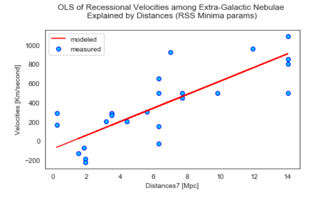
If we compare this scatter plot to the one we generated earlier during EDA, there’s a slight difference as the red line is a bit steeper. It doesn’t pass through the second galaxy from the top at 14 Mpc but rather is slightly above it. We can consider this an improvement in the overall fit of the model!

如果將散布圖與我們在EDA期間生成的散布圖進行比較，則會有一點差異，因為紅線更陡一些。 它沒有以14 Mpc的速度從頂部穿過第二個星系，而是略高于它。 我們可以認為這是模型整體擬合的改進！

In the final section, we will conduct a hypothesis test to examine the theory that the length of galactic distance from Earth has an effect on the galaxy’s recessional velocity. We’ve already used a number of tools in our hacker stats toolbox to examine Hubble’s Law. Let’s put the finishing touches on the icing of the cake!

在最后一節中，我們將進行假設檢驗，以檢驗銀河系與地球之間的距離長度對銀河系的后退速度有影響的理論。 我們已經在黑客統計信息工具箱中使用了許多工具來檢查哈勃定律。 讓我們為蛋糕錦上添花！

假設檢驗→銀河星云的距離是否對其后退速度有觀察到的影響？ (Hypothesis Test → Do the distances of galactic nebulae have an observed effect on their recession velocities?)

Recall that we used the assumption of the central limit theorem to generate enough replicates to obtain paired resampled normal distributions of galactic distances and recessional velocities. Data that is normally distributed is one of the assumptions required for a hypothesis test.

回想一下，我們使用中心極限定理的假設來生成足夠的重復項，以獲得成對的重新采樣的銀河距離和后退速度正態分布。 正態分布的數據是假設檢驗所需的假設之一。

Now we will test whether the length of galactic distance has an observed effect on recessional velocity. We will define short and long distances of galaxies from planet Earth. Then we will resample and shuffle the velocities and take the difference in resampled means as a test statistic. In other words, if the test statistic distribution truly exhibits a difference in effect (ie. mean difference of velocities > 0 ) then we can reject the null hypothesis, and conclude with enough power that the results are statistically significant.

現在，我們將測試銀河距離的長度是否對后退速度有觀察到的影響。 我們將定義星系與地球之間的短距離和長距離。 然后，我們將對速度進行重新采樣和改組，并將重新采樣的均值之差作為檢驗統計量。 換句話說，如果檢驗統計量分布確實顯示出效果上的差異(即，速度的平均差異> 0)，那么我們可以拒絕原假設，并以足夠的能力得出結論，該結果在統計上是有意義的。

See the null and alternative hypotheses below:

請參見下面的原假設和替代假設：

Null Hypothesis

零假設

• The length of distance has no effect on the recession velocity of Extra-Galactic Nebulae.

  距離的長度對銀河外星云的后退速度沒有影響。

Alternative Hypothesis

替代假設

• The length of distance has an observed effect on the recession velocity velocities of Extra-Galactic Nebulae.

  距離的長度對銀河外星云的后退速度有影響。

Assumptions

假設條件

For our experiment, we will use a 95% significance level, which will make our alpha value 0.05. We define short distances as distances less than 7 Mpc; Conversely, we define long distances as distances that are greater or equal to 7 Mpc → Note that this will be done with our adjusted values for distances.

對于我們的實驗，我們將使用95％的顯著性水平，這將使我們的alpha值為0.05。 我們將短距離定義為小于7 Mpc的距離； 相反，我們將長距離定義為大于或等于7 Mpc的距離→請注意，這將通過我們對距離的調整值來完成。

We’re going to use a T-test since we do not know the true standard deviation of the population; We will use 1,000 bootstrap replicates of galactic recessional velocities.

因為我們不知道總體的真實標準偏差，所以我們將使用T檢驗。 我們將使用1,000個銀河衰退速度的自舉復制。

The test statistic is the difference between a recession velocity drawn from shorter distances and one drawn from longer distances. The distribution of difference values is built up by subtracting each point in the shorter range with one from the longer range, to see if the mean difference is greater than zero, also known as the effect size.

檢驗統計量是從較短距離得出的衰退速度與從較長距離得出的衰退速度之差。 差值的分布是通過將較短范圍內的每個點減去較長范圍中的一個點而建立的，以查看平均差是否大于零(也稱為效果大小)。

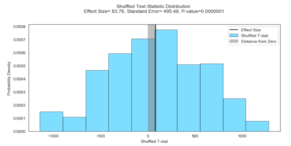
And there we have it! The mean of the test statistic is not zero (denoted by the shaded region in gray), which tells us that there is on average an 83.76 km per second difference in velocities when comparing short and long galactic distances. Again, we refer to this as our effect size. In other words, galaxies that are closer to Earth are moving away at a much slower rate than galaxies that are a lot further away from Earth. The increase in the galactic distance from Earth had an observed effect on recessional velocity. The standard error of the test statistic distribution is also not zero, so there is uncertainty in the size of the effect.

我們終于得到它了！ 測試統計的平均值不為零(由灰色陰影區域表示)，這告訴我們在比較短銀河和長銀河距離時平均每秒速度相差83.76 km。 同樣，我們將此稱為效應大小。 換句話說，離地球更近的星系的移動速度比離地球更遠的星系移動的速度要慢得多。 到地球的銀河距離的增加對后退速度有觀察到的影響。 測試統計量分布的標準誤差也不是零，因此影響的大小存在不確定性。

It’s also worthwhile to mention that shuffling the resampled data points had an effect on the randomness of our experiment. We shuffled the data in order to make sure that each sample is composed of random and independent data points, which are other assumptions required for a hypothesis test. If we didn’t shuffle the data then the effect size would be much greater due to the time-ordered effect on the mean.

還值得一提的是，對重新采樣的數據點進行混洗會影響我們實驗的隨機性。 我們對數據進行了混洗，以確保每個樣本均由隨機和獨立的數據點組成，這是假設檢驗所需的其他假設。 如果我們不對數據進行混洗，那么由于均值的時間順序影響，影響大小會更大。

Finally, our P-value is extremely small → 0.0000001

最后，我們的P值非常小→0.0000001

Thus, we can conclude with a high degree of statistical significance that the distances of galaxies from Earth have an effect on their recessional velocities, which is observational evidence of Hubble’s Law. The universe is constantly expanding all around us!

因此，我們可以得出具有高度統計意義的結論，即星系與地球的距離會影響它們的后退速度，這是哈勃定律的觀測證據。 宇宙不斷在我們周圍擴展！

P.S. ~ Note that we didn’t use power analysis to determine the sample size for the hypothesis test upfront, since we weren’t privy to the standard effect size at the beginning of the experiment. According to traditional stats textbooks, one should determine the needed sample size prior to performing a hypothesis test. Instead, we opted for the hacker stats approach: we ran a hypothesis test with 1,000 samples, retrieved the effect size and standard error of the effect, and hacked the needed sample size. The result was roughly 910 observations, which worked well in our favor. Got to love hacker stats!

PS?請注意，由于我們在實驗開始時并不熟悉標準效應量，因此我們并未使用功效分析來預先確定假設檢驗的樣本量。 根據傳統的統計教科書，應該在執行假設檢驗之前確定所需的樣本量。 相反，我們選擇了黑客統計方法：我們對1,000個樣本進行了假設檢驗，檢索了效應大小和效應的標準誤，然后黑客入侵了所需的樣本量。 結果大約是910個觀測值，對我們有利。 愛上了黑客統計信息！

下一步 (Next Steps)

• Add 22 estimated distances for the T-test.
  為T檢驗加上22個估計的距離。
• Identify Nebulae Clusters with KMeans.
  用KMeans識別星云團。
• Use other data sources of galactic distances & recession velocities…
  使用銀河距離和后退速度的其他數據源…

We could have used the 22 estimated distances for our T-test as well, bringing the total number of observations up to 46.

我們也可以將22個估計的距離用于T檢驗，從而使觀測的總數達到46個。

Hubble grouped the 24 galaxies into 9 clusters. This would be an interesting exercise to see if we get the same cluster centroids with KMeans or Agglomerative clustering.

哈勃將24個星系分為9個星團。 看看我們是否獲得具有KMeans或聚集聚類的相同聚類質心，這將是一個有趣的練習。

Finally, we can also use data from the Hubble telescope to examine Hubble’s law.

最后，我們還可以使用哈勃望遠鏡的數據檢查哈勃定律。

As Hubble concludes in his PNAS paper, “The results establish a roughly linear relation between velocities and distances among nebulae for which velocities have been previously published, and the [relationship] appears to dominate the distribution of velocities…..New data to be expected in the near future may modify the significance of the present investigation or, if confirmatory, will lead to a solution many times the weight.” (1)

正如哈勃在其PNAS論文中總結的那樣：“結果建立了速度與星云之間的距離之間的大致線性關系，先前已經針對該距離發布了速度，[關系]似乎主導了速度的分布……..新數據有望得到預料在不久的將來可能會改變當前調查的意義，或者，如果證實這一點，將導致解決方案的重量增加很多倍。” (1)