Video Link

影片連結

You can view the code used in this Episode here: SampleCode

您可以在此處查看 此劇 集中使用的代碼： SampleCode

導入我們的數據 (Importing our Data)

The first step is to import our data into python.

第一步是將我們的數據導入python。

We can do that by going on the following link: Data

我們可以通過以下鏈接來做到這一點： 數據

Click on “code” and download ZIP.

單擊“代碼”并下載ZIP。

Locate WeatherDataP.csv and copy it into your local disc under a new file called ProjectData

找到WeatherDataP.csv并將其復制到本地磁盤下名為ProjectData的新文件下

Note: WeatherData.csv and WeahterDataM.csv were used in Simple Linear Regression and Multiple Linear Regression.

注意：WeatherData.csv和WeahterDataM.csv用于簡單線性回歸和多重線性回歸 。

Now we are ready to import our data into our Notebook:

現在我們準備將數據導入到筆記本中：

How to set up a new Notebook can be found at the start of Episode 4.3

如何設置新筆記本可以在第4.3節開始時找到

Note: Keep this medium post on a split screen so you can read and implement the code yourself.

注意：請將此帖子張貼在分屏上，以便您自己閱讀和實現代碼。

# Import Pandas Library, used for data manipulation
# Import matplotlib, used to plot our data
# Import numpy for linear algebra operationsimport pandas as pd
import matplotlib.pyplot as plt
import numpy as np# Import our WeatherDataP.csv and store it in the variable rweather_data_pweather_data_p = pd.read_csv("D:\ProjectData\WeatherDataP.csv") 
# Display the data in the notebookweather_data_p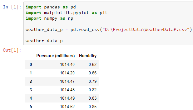

繪制數據 (Plotting our Data)

In order to check what kind of relationship Pressure forms with Humidity, we plot our two variables.

為了檢查壓力與濕度之間的關系，我們繪制了兩個變量。

# Set our input x to Pressure, use [[]] to convert to 2D array suitable for model inputX = weather_data_p[["Pressure (millibars)"]]
y = weather_data_p.Humidity# Produce a scatter graph of Humidity against Pressureplt.scatter(X, y, c = "black")
plt.xlabel("Pressure (millibars)")
plt.ylabel("Humidity")

Here we see Humidity vs Pressure forms a bowl shaped relationship, reminding us of the function: y = 𝑥2 .

在這里，我們看到濕度與壓力之間呈碗形關系，使我們想起了函數y =𝑥2。

預處理我們的數據 (Preprocessing our Data)

This is the additional step we apply to polynomial regression, where we add the feature 𝑥2 to our Model.

這是我們應用于多項式回歸的附加步驟 ，在此步驟中將特征𝑥2添加到模型中。

# Import the function "PolynomialFeatures" from sklearn, to preprocess our data
# Import LinearRegression model from sklearnfrom sklearn.preprocessing import PolynomialFeatures
from sklearn.linear_model import LinearRegression# Set PolynomialFeatures to degree 2 and store in the variable pre_process
# Degree 2 preprocesses x to 1, x and x^2
# Degree 3 preprocesses x to 1, x, x^2 and x^3
# and so on..pre_process = PolynomialFeatures(degree=2)# Transform our x input to 1, x and x^2X_poly = pre_process.fit_transform(X)# Show the transformation on the notebookX_poly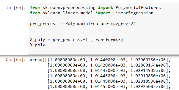

e+.. refers to the position of the decimal place.

e + ..指小數位的位置。

E.g1.0e+00 = 1.0 [ keep the decimal point where it is ]1.0144e+03 = 1014.4 [ Move the decimal place 3 places to the right ]1.02900736e+06 = 1029007.36 [ Move the decimal place 6 to places to the right ]

例如 1.0e + 00 = 1.0 [保留小數點處的位置] 1.0144e + 03 = 1014.4 [將小數位右移3位] 1.02900736e + 06 = 1029007.36 [將小數點6向右移動]

— — — — — — — — — — — — — — — — — —

— — — — — — — — — — — — — — — — — — — —

The code above makes the following Conversion:

上面的代碼進行了以下轉換：

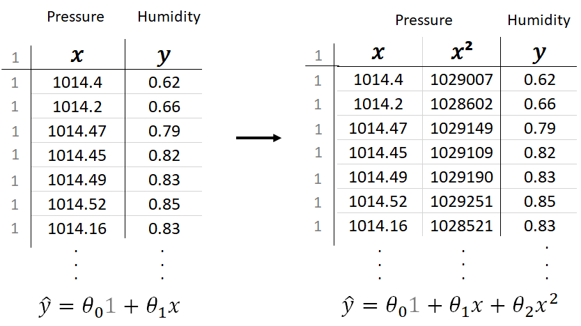
Notice that there is a hidden column of 1’s which can be thought of as the variable associated with θ?. Since θ? × 1 = θ? this is often left out.

請注意，有一個隱藏的1列，可以將其視為與θ?相關的變量。 由于θ?×1 =θ?，因此經常被忽略。

— — — — — — — — — — — — — — — — — —

— — — — — — — — — — — — — — — — — — — —

實現多項式回歸 (Implementing Polynomial Regression)

The method here remains the same as multiple linear regression in python, but here we are fitting our regression model to the preprocessed data:

此處的方法與python中的多元線性回歸相同，但此處我們將回歸模型擬合為預處理的數據：

pr_model = LinearRegression()# Fit our preprocessed data to the polynomial regression modelpr_model.fit(X_poly, y)# Store our predicted Humidity values in the variable y_newy_pred = pr_model.predict(X_poly)# Plot our model on our dataplt.scatter(X, y, c = "black")
plt.xlabel("Pressure (millibars)")
plt.ylabel("Humidity")
plt.plot(X, y_pred)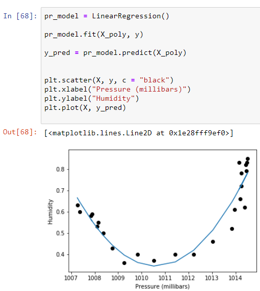

We can extract θ?, θ? and θ? using the following code:

我們可以使用以下代碼提取θ?，θ?和θ2 ：

theta0 = pr_model.intercept_
_, theta1, theta2 = pr_model.coef_theta0, theta1, theta2

A “_” is used to ignore the first value in pr_model.coef as this is given by default as 0. The other two co-efficients are labelled theta1 and theta 2 respectively.

“ _”用于忽略pr_model.coef中的第一個值，因為默認情況下該值為0。其他兩個系數分別標記為theta1和theta 2。

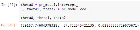
Giving our polynomial regression model roughly as:

大致給出我們的多項式回歸模型：

使用我們的回歸模型進行預測 (Using our Regression Model to make predictions)

# Predict humidity for a pressure of 1007 millibars
# Tranform 1007 to 1, 1007, 1007^2 suitable for input, using 
# pre_process.fit_transformy_new = pr_model.predict(pre_process.fit_transform([[1007]]))
y_new

Here we expect a Humidity value of 0.7164631 for a pressure reading of 1007 millibars.

在這里，對于1007毫巴的壓力讀數，我們期望的濕度值為0.7164631。

We can plot this point on our data plot using the following code:

我們可以使用以下代碼在數據圖上繪制該點：

plt.scatter(1007, y_new, c = "red")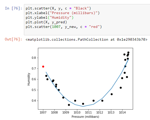

評估我們的模型 (Evaluating our Model)

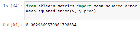
To evaluate our model we are going to be using mean squared error (MSE), discussed in the previous episode, the function can easily be imported from sklearn.

為了評估我們的模型，我們將使用上一集中討論的均方誤差(MSE) ，可以輕松地從sklearn導入函數。

from sklearn.metrics import mean_squared_error
mean_squared_error(y, y_pred)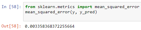

The mean squared error for our regression model is given by: 0.003358..

我們的回歸模型的均方誤差為：0.003358 ..

If we want to change our model to include 𝑥3 we can do so by simply changing PolynomialFeatures to degree 3:

如果要更改模型以包括𝑥3 ，可以通過將PolynomialFeatures更改為3級來實現 ：

pre_process = PolynomialFeatures(degree=3)

Let’s check if this has decreased our mean squared error:

讓我們檢查一下這是否降低了均方誤差：

Indeed it has.

確實有。

You can change the degree used in PolynomialFeatures to anything you like and see for yourself what effect this has on our MSE.

您可以將PolynomialFeatures中使用的度數更改為您喜歡的任何值，并親自查看這對我們的MSE有什么影響。

Ideally we want to choose the model that:

理想情況下，我們要選擇以下模型：

• Has the lowest MSE

  MSE最低

• Does not over-fit our data

  不會過度擬合我們的數據

It is important that we plot our model on our data to ensure we don’t end up with the model shown at the end of Episode 4.6, which had an extremely low MSE but over-fitted our data.

重要的是， 我們需要在數據上繪制模型，以確保最終不會出現第4.6集末顯示的模型，該模型的MSE極低，但數據過擬合。

上一集 - 下一集 (Prev Episode — Next Episode)

如有任何疑問，請留在下面！ (If you have any questions please leave them below!)