The goal of this challenge is to predict whether a customer will make a transaction (“target” = 1) or not (“target” = 0). For that, we get a data set of 200 incognito variables and our submission is judged based on the Area Under Receiver Operating Characteristic Curve which we have to maximise.

這項挑戰的目的是預測客戶是否會進行交易(“目標” = 1)(“目標” = 0)。 為此，我們獲得了200個隱身變量的數據集，并根據必須最大化的接收器工作特征曲線下面積來判斷提交。

This project is somewhat different from others, you basically get a huge amount of data with no missing values and only numbers. A dream come true for any data scientist. Of course, that sounds too good to be true! Let’s dive in.

這個項目與其他項目有些不同，您基本上可以獲得大量的數據，沒有缺失值，只有數字。 任何數據科學家都夢想成真。 當然，這聽起來好得令人難以置信！ 讓我們潛入。

一，設置 (I. Set up)

We start by loading the data and get a quick overview of the data we’ll have to handle. We do so by calling the describe() and info() functions.

我們首先加載數據，然后快速概覽需要處理的數據。 我們通過調用describe()和info()函數來實現。

# Load the data setstrain_df = pd.read_csv("train.csv")
test_df = pd.read_csv("test.csv")# Create a merged data set and review initial informationcombined_df = pd.concat([train_df, test_df])
print(combined_df.describe())
print(combined_df.info())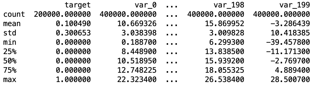

We have a total of 400.000 observations, 200.000 of whom in our training set. We can also see that we will have to deal with the class imbalance issue as we have a mean of 0.1 in the target column.

我們總共有400.000個觀測值，其中有200.000個在我們的訓練集中。 我們還可以看到，我們必須處理類不平衡問題，因為目標列的平均值為0.1。

二。 缺失值 (II. Missing values)

Let’s check whether we have any missing values. For that, we print the column names that contain missing values.

讓我們檢查是否缺少任何值。 為此，我們打印包含缺少值的列名稱。

# Check missing valuesprint(combined_df.columns[combined_df.isnull().any()])

We have zero missing values. Let’s move forward.

我們的零缺失值。 讓我們前進。

三， 資料類型 (III. Data types)

Let’s check the data we have. Are we dealing with categorical variables? Or text? Or just numbers? We print a dictionary containing the different types of data we have and its occurrence.

讓我們檢查一下我們擁有的數據。 我們在處理分類變量嗎？ 還是文字？ 還是數字？ 我們打印一個字典，其中包含我們擁有的不同數據類型及其出現的位置。

# Get the data typesprint(Counter([combined_df[col].dtype for col in combined_df.columns.values.tolist()]).items())

Only float data. We don’t have to create dummy variables.

僅浮動數據。 我們不必創建虛擬變量。

IV。 數據清理 (IV. Data cleaning)

We don’t want to use our ID column to make our predictions and therefore store it into the index.

我們不想使用ID列進行預測，因此將其存儲到索引中。

# Set the ID col as indexfor element in [train_df, test_df]:
    element.set_index('ID_code', inplace = True)

We now separate the target variable from our training set and create a new dataframe for our target variable.

現在，我們將目標變量從訓練集中分離出來，并為目標變量創建一個新的數據框。

# Create X_train_df and y_train_df setX_train_df = train_df.drop("target", axis = 1)
y_train_df = train_df["target"]

V.縮放 (V. Scaling)

We haven’t done anything when it comes to data exploration and outlier analysis. It is always highly recommended to conduct these. However, given the nature of the challenge, we suspect that the variables in themselves might not be too interesting.

在數據探索和離群值分析方面，我們沒有做任何事情。 始終強烈建議進行這些操作。 但是，鑒于挑戰的性質，我們懷疑變量本身可能不太有趣。

In order to compensate for our lack of outlier detection, we scale the data using RobustScaler().

為了彌補我們對異常值檢測的不足，我們使用RobustScaler()縮放數據。

# Scale the data and use RobustScaler to minimise the effect of outliersscaler = RobustScaler()# Scale the X_train setX_train_scaled = scaler.fit_transform(X_train_df.values)
X_train_df = pd.DataFrame(X_train_scaled, index = X_train_df.index, columns= X_train_df.columns)# Scale the X_test setX_test_scaled = scaler.transform(test_df.values)
X_test_df = pd.DataFrame(X_test_scaled, index = test_df.index, columns= test_df.columns)

We now create a X_train, y_train, X_test and y_test set for training our model and then testing it on hold-out data.

現在，我們創建一個X_train，y_train，X_test和y_test集來訓練我們的模型，然后對保留數據進行測試。

# Split our training sample into train and test, leave 20% for testX_train, X_test, y_train, y_test = train_test_split(X_train_df, y_train_df, test_size=0.2, random_state = 20)

When it comes to outliers, some could use IsolationForest() in order to automatically identify and remove rows that are outliers. This technique is often used for data sets with numerous variables. This code chunk has been borrowed form MachineLearningMastery.

當涉及到離群值時，有些人可以使用IsolationForest()來自動識別和刪除離群值。 此技術通常用于具有眾多變量的數據集。 該代碼塊已從MachineLearningMastery借用。

# OUTLIERS# Remove outliers automaticallyiso = IsolationForest(contamination=0.1)
yhat = iso.fit_predict(X_train)
print(yhat)# Select all rows that are not outliersmask = yhat != -1
X_train, y_train = X_train.loc[mask, :], y_train.loc[mask]

Please note that this automated outlier discovery did not add any predictive power to our model and we decided to comment it out.

請注意，這種自動化的異常值發現并未為我們的模型增加任何預測能力，因此我們決定將其注釋掉。

七。 班級失衡 (VII. Class Imbalance)

In our data, we have seen that we have way less observations that have made a transaction than have not. If we want our model to be equally capable at predicting both, we should make sure we don’t feed it with skewed data.

在我們的數據中，我們已經看到，進行交易的觀察少于未觀察到的觀察。 如果我們希望我們的模型能夠同時預測兩者，則應確保不向其提供偏斜的數據。

We correct for class imbalance by upsampling the minority class. This techniques are inspired from this excellent article by Tara Boyle.

我們通過增加少數族裔的樣本來糾正階級失衡。 該技術的靈感來自Tara Boyle的這篇出色文章 。

# CLASS IMBALANCE# Downsample majority class# Concatenate our training data back togetherX = pd.concat([X_train, y_train], axis=1)# Separate minority and majority classesnot_transa = X[X.target==0]
transa = X[X.target==1]
not_transa_down = resample(not_transa,
                                replace = False, # sample without replacementn_samples = len(transa), # match minority nrandom_state = 27) # reproducible results# Combine minority and downsampled majoritydownsampled = pd.concat([not_transa_down, transa])# Checking countsprint(downsampled.target.value_counts())# Create training set againy_train = downsampled.target
X_train = downsampled.drop('target', axis=1)
print(len(X_train))

Here is the code for upsampling the minority class.

這是對少數群體進行升采樣的代碼。

# Upsample minority class# Concatenate our training data back togetherX = pd.concat([X_train, y_train], axis=1)# Separate minority and majority classesnot_transa = X[X.target==0]
transa = X[X.target==1]
not_transa_up = resample(transa,
                                replace = True, # sample without replacementn_samples = len(not_transa), # match majority nrandom_state = 27) # reproducible results# Combine minority and downsampled majorityupsampled = pd.concat([not_transa_up, not_transa])# Checking countsprint(upsampled.target.value_counts())# Create training set againy_train = upsampled.target
X_train = upsampled.drop('target', axis=1)
print(len(X_train))

And here is the code for creating synthetic samples with SMOTE.

這是使用SMOTE創建合成樣本的代碼。

# Create synthetic samplessm = SMOTE(random_state=27, sampling_strategy='minority')
X_train, y_train = sm.fit_sample(X_train, y_train)
print(y_train.value_counts())

八。 造型 (VIII. Modelling)

We now dive deeper into the models. The plan is to create 4 different models and then averaging their predictions to make an ensemble that will yield the final prediction. We do not plan to fine tune the models to a too wide extent. Leaving GridSearch out of this.

現在，我們深入研究模型。 計劃是創建4個不同的模型，然后對它們的預測取平均，以形成一個可以產生最終預測的集合。 我們不打算對模型進行微調。 將GridSearch排除在外。

1. Keras神經網絡 (1. Neural Network With Keras)

# NEURAL NETWORK# Build our neural network with input dimension 200classifier = Sequential()# First Hidden Layerclassifier.add(Dense(150, activation='relu', kernel_initializer='random_normal', input_dim=200))# Second  Hidden Layerclassifier.add(Dense(350, activation='relu', kernel_initializer='random_normal'))# Third  Hidden Layerclassifier.add(Dense(250, activation='relu', kernel_initializer='random_normal'))# Fourth  Hidden Layerclassifier.add(Dense(50, activation='relu', kernel_initializer='random_normal'))# Output Layerclassifier.add(Dense(1, activation='sigmoid', kernel_initializer='random_normal'))# Compile the networkclassifier.compile(optimizer ='adam',loss='binary_crossentropy', metrics =['accuracy'])# Fitting the data to the training data setclassifier.fit(X_train,y_train, batch_size=100, epochs=150)# Evaluate the model on training dataeval_model=classifier.evaluate(X_train, y_train)
print(eval_model)# Make predictions on the hold out datay_pred=classifier.predict(X_test)
y_pred =(y_pred>0.5)# Get the confusion matrixcm = confusion_matrix(y_test, y_pred)
print(cm)# Get the accuracy scoreprint("Accuracy of {}".format(accuracy_score(y_test, y_pred)))# Get the f1-Scoreprint("f1 score of {}".format(f1_score(y_test, y_pred)))# Get the recall scoreprint("Recall score of {}".format(recall_score(y_test, y_pred)))# Make predictions and create submission filepredictions = (classifier.predict(X_test_df)>0.5)
predictions = np.concatenate(predictions, axis=0 )
my_pred = pd.DataFrame({'ID_code': X_test_df.index, 'target': predictions})# Set 0 and 1s instead of True and Falsemy_pred["target"] = my_pred["target"].map({True:1, False : 0})# Create CSV filemy_pred.to_csv('pred_ann.csv', index=False)

This model is built upon the excellent review from Renu Khandelwal. We haven’t modified the original script except adding some layers and increased the number of neurons by layer.

該模型基于Renu Khandelwal的出色評論 。 除了添加一些層并逐層增加神經元的數量外，我們沒有修改原始腳本。

Our first submission with this Neural Network gives us a score of 0.80882

我們在該神經網絡中的首次提交給我們得分0.80882

2. LightGBM (2. LightGBM)

# LIGHT GBM# Get the train and test data for the training sequencetrain_data = lgbm.Dataset(X_train, label=y_train)
test_data = lgbm.Dataset(X_test, label=y_test)# Set parameters
parameters = {'application': 'binary','objective': 'binary','metric': 'auc','is_unbalance': 'true','boosting': 'gbdt','num_leaves': 31,'feature_fraction': 0.5,'bagging_fraction': 0.5,'bagging_freq': 20,'learning_rate': 0.05,'verbose': 0
}# Train our classifier
classifier = lgbm.train(parameters,
                       train_data,
                       valid_sets= test_data,
                       num_boost_round=5000,
                       early_stopping_rounds=100)# Make predictionspredictions = classifier.predict(X_test_df.values)# Create submission filemy_pred_lgbm = pd.DataFrame({'ID_code': X_test_df.index, 'target': predictions})# Create CSV filemy_pred_lgbm.to_csv('pred_lgbm.csv', index=False)

This code chunk is based on some work from this Kaggle Notebook by E. Zietsman. If you want a complete overview of how LightGBM works and how to optimally tune it, make sure you read this article from Pushkar Mandot.

此代碼塊基于E. Zietsman的Kaggle筆記本所做的一些工作。 如果要全面了解LightGBM的工作原理以及如何對其進行最佳調整，請確保您閱讀了Pushkar Mandot的 這篇文章 。

This gives us a score of 0.89217

這給了我們0.89217的分數

3. XGBoost (3. XGBoost)

# XGBOOST# Instantiate classifierclassifier = XGBClassifier(
    tree_method = 'hist',
    objective = 'binary:logistic',
    eval_metric = 'auc',
    learning_rate = 0.01,
    max_depth = 2,
    colsample_bytree = 0.35,
    subsample = 0.8,
    min_child_weight = 53,
    gamma = 9,
    silent= 1)# Fit the dataclassifier.fit(X_train, y_train)# Make predictions on the hold out datay_pred = (classifier.predict_proba(X_test)[:,1] >= 0.5).astype(int)# Get the confusion matrixprint(confusion_matrix(y_test, y_pred))# Get the accuracy scoreprint("Accuracy of {}".format(accuracy_score(y_test, y_pred)))# Get the f1-Scoreprint("f1 score of {}".format(f1_score(y_test, y_pred)))# Get the recall scoreprint("Recall score of {}".format(recall_score(y_test, y_pred)))# Make predictionspredictions = (classifier.predict_proba(X_test_df)[:,1] >= 0.5).astype(int)# Create submission filemy_pred_xgb = pd.DataFrame({'ID_code': X_test_df.index, 'target_xgb': predictions})# Create CSV filemy_pred_xgb.to_csv('pred_xgb.csv', index=False)

We also rely on XGBoost and the helpfull insights from Félix Revert.

我們還依靠XGBoost和有益的見解 ，從費利克斯還原 。

This gives us a score of 0.59283

這使我們得到0.59283的分數

4. Catboost (4. Catboost)

# CATBOOST# Instantiate classifierclassifier = cb.CatBoostClassifier(loss_function="Logloss",
                           eval_metric="AUC",
                           learning_rate=0.01,
                           iterations=1000,
                           random_seed=42,
                           od_type="Iter",
                           depth=10,
                           early_stopping_rounds=500
                          )# Fit the dataclassifier.fit(X_train, y_train)# Make predictions on the hold out datay_pred = (classifier.predict_proba(X_test)[:,1] >= 0.5).astype(int)# Get the confusion matrixprint(confusion_matrix(y_test, y_pred))# Get the accuracy scoreprint("Accuracy of {}".format(accuracy_score(y_test, y_pred)))# Get the f1-Scoreprint("f1 score of {}".format(f1_score(y_test, y_pred)))# Get the recall scoreprint("Recall score of {}".format(recall_score(y_test, y_pred)))# Make predictionspredictions = (classifier.predict_proba(X_test_df)[:,1] >= 0.5).astype(int)# Create submission filemy_pred_cat = pd.DataFrame({'ID_code': X_test_df.index, 'target_cat': predictions})# Create CSV filemy_pred_cat.to_csv('pred_cat.csv', index=False)

This part is inspired from Wakame on Kaggle.

這部分靈感來自Kaggle上的Wakame 。

This gives us a score of 0.78769

這給予我們0.78769的分數

5.合奏 (5. Ensemble)

In this last part, we take the 4 models we created and ensemble them in order to generate our final answer. We want at least 3 out of the 4 models to qualify an observation as 1 in order to effectively doing so.

在最后一部分中，我們將使用我們創建的4個模型并將它們集成在一起以生成最終答案。 為了有效地做到這一點，我們希望4個模型中至少有3個將觀察結果定為1。

# ENSEMBLE# Create data framemy_pred_ens = pd.concat([my_pred_ann, my_pred_xgb, my_pred_cat, my_pred_lgbm], axis = 1, sort=False)# Review our frameprint(my_pred_ens.describe())# Sum all the predictions and only assign a 1 if sum is higher than 2my_pred_ens["target"] = my_pred_ens["target_ann"] + my_pred_ens["target_xgb"] + my_pred_ens["target_lgbm"] + my_pred_ens["target_cat"]# Assign a 1 if sum is higher than 2my_pred_ens["target"] = np.where(my_pred_ens["target"] > 2, 1, 0)# Remove other target colsmy_pred_ens = my_pred_ens.drop(["target_ann", "target_lgbm", "target_xgb", "target_cat"], axis = 1)# Create submission filemy_pred = pd.DataFrame({'ID_code': X_test_df.index, 'target': my_pred_ens["target"]})# Create CSV filemy_pred.to_csv('pred_ens.csv', index=False)

This gives us a score of 0.78627

這給了我們0.78627的分數

九。 結論 (IX. Conclusion)

Our best models was the LightGBM. In order to improve on our score, we might rely on Stratified Kfolds or any other cross validation technique. We might as well fine tune our models in more detail.

我們最好的模型是LightGBM。 為了提高我們的分數，我們可能依賴于Stratified Kfolds或任何其他交叉驗證技術。 我們不妨更詳細地調整模型。

使用的包 (Packages used)

import pandas as pdimport numpy as npfrom collections import Counterfrom sklearn.preprocessing import RobustScalerfrom sklearn.model_selection import train_test_splitfrom keras import Sequentialfrom keras.layers import Densefrom sklearn.metrics import confusion_matrix, accuracy_score, recall_score, f1_score, roc_curve, roc_auc_scorefrom sklearn.utils import resampleimport lightgbm as lgbmfrom xgboost import XGBClassifierfrom sklearn import metricsfrom sklearn.model_selection import GridSearchCVfrom sklearn.ensemble import IsolationForestfrom imblearn.over_sampling import SMOTEfrom sklearn.model_selection import StratifiedKFoldimport xgboost as xgbimport catboost as cbfrom catboost import Poolfrom sklearn.model_selection import KFold

我們從中汲取了靈感的有用資源 (Helpful sources we drew inspiration from)