袋裝樹木介紹 (Introduction to Bagged Trees)

Without diving into the specifics just yet, it’s important that you have some foundation understanding of decision trees.

尚未深入研究細節，對決策樹有一定基礎了解就很重要。

From the evaluation approach of each algorithm to the algorithms themselves, there are many similarities.

從每種算法的評估方法到算法本身，都有很多相似之處。

If you aren’t already familiar with decision trees I’d recommend a quick refresher here.

如果您還不熟悉決策樹，我建議在這里快速復習。

With that said, get ready to become a bagged tree expert! Bagged trees are famous for improving the predictive capability of a single decision tree and an incredibly useful algorithm for your machine learning tool belt.

話雖如此，準備成為袋裝樹專家！ 袋裝樹以提高單個決策樹的預測能力和對您的機器學習工具帶非常有用的算法而聞名。

什么是袋裝樹？什么使它們如此有效？ (What are Bagged Trees & What Makes Them So Effective?)

為什么要使用袋裝樹木 (Why use bagged trees)

The main idea between bagged trees is that rather than depending on a single decision tree, you are depending on many many decision trees, which allows you to leverage the insight of many models.

套袋樹之間的主要思想是，您不依賴于單個決策樹，而是依賴于許多決策樹，這使您可以利用許多模型的洞察力。

偏差偏差的權衡 (Bias-variance trade-off)

When considering the performance of a model, we often consider what’s known as the bias-variance trade-off of our output. Variance has to do with how our model handles small errors and how much that potentially throws off our model and bias results in under-fitting. The model effectively makes incorrect assumptions around the relationships between variables.

在考慮模型的性能時，我們經常考慮所謂的輸出偏差-偏差權衡。 方差與我們的模型如何處理小錯誤以及與模型的潛在偏離和導致擬合不足的偏差有關。 該模型有效地圍繞變量之間的關系做出了錯誤的假設。

You could say the issue with variation is while your model may be directionally correct, it’s not very accurate, while if your model is very biased, while there could be low variation; it could be directionally incorrect entirely.

您可以說變化的問題在于，模型可能在方向上是正確的，但不是很準確；而如果模型有很大偏差，那么變化可能就很小。 它可能完全是方向錯誤的。

The biggest issue with a decision tree, in general, is that they have high variance. The issue this presents is that any minor change to the data can result in major changes to the model and future predictions.

通常，決策樹的最大問題是它們的差異很大。 這帶來的問題是，數據的任何細微變化都可能導致模型和未來預測的重大變化。

The reason this comes into play here is that one of the benefits of bagged trees, is it helps minimize variation while holding bias consistent.

之所以在這里發揮作用，是因為袋裝樹木的好處之一是，它可以在保持偏差一致的同時最大程度地減少變化。

為什么不使用袋裝樹木 (Why not use bagged trees)

One of the main issues with bagged trees is that they are incredibly difficult to interpret. In the decision trees lesson, we learned that a major benefit of decision trees is that they were considerably easier to interpret. Bagged trees prove the opposite in this regard as its process lends to complexity. I’ll explain that more in-depth shortly.

套袋樹的主要問題之一是難以解釋。 在決策樹課程中，我們了解到決策樹的主要好處是它們易于解釋。 袋裝樹在這方面被證明是相反的，因為其過程增加了復雜性。 我將在短期內更深入地解釋。

什么是裝袋？ (What is bagging?)

Bagging stands for Bootstrap Aggregation; it is what is known as an ensemble method — which is effectively an approach to layering different models, data, algorithms, and so forth.

Bagging代表Bootstrap聚合； 這就是所謂的集成方法，實際上是一種對不同模型，數據，算法等進行分層的方法。

So now you might be thinking… ok cool, so what is bootstrap aggregation…

所以現在您可能在想……好極了，那么引導聚合是什么……

What happens is that the model will sample a subset of the data and will train a decision tree; no different from a decision tree so far… but what then happens is that additional samples are taken (with replacement — meaning that the same data can be included multiple times), new models are trained, and then the predictions are averaged. A bagged tree could include 5 trees, 50 trees, 100 trees and so on. Each tree in your ensemble may have different features, terminal node counts, data, etc.

發生的事情是該模型將對數據的一個子集進行采樣并訓練決策樹。 到目前為止，它與決策樹沒有什么不同……但是接下來發生的是，將額外取樣(進行替換-意味著可以多次包含相同的數據)，訓練新模型，然后對預測取平均。 袋裝樹可以包括5棵樹，50棵樹，100棵樹等等。 集合中的每棵樹可能具有不同的功能，終端節點數，數據等。

As you can imagine, a bagged tree is very difficult to interpret.

可以想象，袋裝樹很難解釋。

訓練袋裝樹 (Train a Bagged Tree)

To start off, we’ll break out our training and test sets. I’m not going to talk much about the train test split here. We’ll be doing this with the Titanic dataset from the titanic package

首先，我們將介紹我們的培訓和測試集。 在這里，我不會談論太多有關火車測試的內容。 我們將使用titanic包中的Titanic數據集進行此操作

n <- nrow(titanic_train)n_train <- round(0.8 * n)set.seed(123) 
train_indices <- sample(1:n, n_train) 
train <- titanic_train[train_indices, ] 
test <- titanic_train[-train_indices, ]

Now that we have our train & test sets broken out, let’s load up the ipred package. This will allow us to run the bagging function.

現在我們有了訓練和測試集，現在讓我們加載ipred包。 這將使我們能夠運行裝袋功能。

A couple things to keep in mind is that the formula indicates that we want to understand Survived by (~ ) Pclass + Sex + Age + SibSp + Parch + Fare + Embarked

幾件事情要記住的是，該公式表明我們想了解Survived的( ~ ) Pclass + Sex + Age + SibSp + Parch + Fare + Embarked

From there you can see that we’re using the train dataset to train this model. & finally, you can see this parameter coob. This is confirming whether we'd like to test performance on an out of bag sample.

從那里您可以看到我們正在使用訓練數據集來訓練此模型。 最后，您可以看到此參數coob 。 這證實了我們是否要測試袋裝樣品的性能。

Remember how I said that each tree re-samples the data? Well, that process leaves a handful of records that will never be used to train with & make up an excellent dataset for testing the model’s performance. This process happens within the bagging function, as you'll see when we print the model.

還記得我說過每棵樹重新采樣數據嗎？ 好的，該過程留下了很少的記錄，這些記錄將永遠不會用于訓練并構成用于測試模型性能的出色數據集。 如我們在打印模型時所見，此過程在bagging功能內進行。

library(ipred) 
set.seed(123) 
model <- bagging(formula = Survived ~ Pclass + Sex + Age + SibSp + Parch + Fare + Embarked, data = train, coob = TRUE) 
print(model)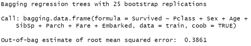

As you can see we trained the default of 25 trees in our bagged tree model.

如您所見，我們在袋裝樹模型中訓練了25棵樹的默認值。

We use the same process to predict for our test set as we use for decision trees.

我們使用與決策樹相同的過程來預測測試集。

pred <- predict(object = model, newdata = test, type = "class") print(pred)

績效評估 (Performance Evaluation)

Now, we’ve trained our model, predicted for our test set, now it’s time to break down different methods of performance evaluation.

現在，我們已經對模型進行了訓練，并針對測試集進行了預測，現在是時候分解不同的性能評估方法了。

ROC曲線和AUC (ROC Curve & AUC)

ROC Curve or Receiver Operating Characteristic Curve is a method for visualizing the capability of a binary classification model to diagnose or predict correctly. The ROC Curve plots the true positive rate against the false positive rate at various thresholds.

ROC曲線或接收器工作特性曲線是一種可視化二進制分類模型正確診斷或預測的功能的方法。 ROC曲線在各種閾值下繪制了真實的陽性率相對于假陽性率。

Our target for the ROC Curve is that the true positive rate is 100% and the false positive rate is 0%. That curve would fall in the top left corner of the plot.

ROC曲線的目標是真實的陽性率為100％，錯誤的陽性率為0％。 該曲線將落在圖的左上角。

AUC is intended to determine the degree of separability, or the ability to correct predict class. The higher the AUC the better. 1 would be perfect, and .5 would be random.

AUC旨在確定可分離性的程度或糾正預測類別的能力。 AUC越高越好。 1將是完美的，而.5將是隨機的。

We’ll be using the metrics package to calculate the AUC for our dataset.

我們將使用metrics包來計算數據集的AUC。

library(Metrics) 
pred <- predict(object = model, newdata = test, type = "prob") auc(actual = test$Survived, predicted = pred[,"yes"])

Here you can see that I change the type to "prob" to return a percentage likelihood rather than the classification. This is needed to calculate AUC.

在這里，您可以看到我將type更改為"prob"以返回百分比可能性而不是分類。 這是計算AUC所必需的。

This returned an AUC of .89 which is not bad at all.

這返回的AUC為0.89，這還算不錯。

截止閾值 (Cut-off Threshold)

In classification, the idea of a cutoff threshold means that given a certain percent likelihood for a given outcome you would classify it accordingly. Wow was that a mouthful. In other words, if you predict survival at 99%, then you’d probably classify it as survival. Well, let’s say you look at another passenger that you predict to survive with a 60% likelihood. Well, they’re still more likely to survive than not, so you probably classify them as survive. When selecting type = "pred" you have the flexibility to specify your own cutoff threshold.

在分類中，閾值閾值的概念意味著給定結果的百分比可能性一定，您就可以對其進行分類。 哇，真是滿嘴。 換句話說，如果您預測生存率為99％，則可能會將其歸類為生存。 好吧，假設您看另一名您預計會以60％的可能性幸存的乘客。 好吧，它們仍然更有可能生存，因此您可能將它們歸類為生存。 選擇type = "pred"您可以靈活地指定自己的截止閾值。

準確性 (Accuracy)

This metric is very simple, what percentage of your predictions were correct. The confusion matrix function from caret includes this.

這個指標非常簡單，您的預測百分比正確無誤。 caret的混淆矩陣函數包括此函數。

混淆矩陣 (Confusion Matrix)

The confusionMatrix function from the caret package is incredibly useful. For assessing classification model performance. Load up the package, and pass it your predictions & the actuals.

caret包中的confusionMatrix函數非常有用。 用于評估分類模型的性能。 加載程序包，并通過它您的預測和實際情況。

library(caret) 
confusionMatrix(data = test$pred, reference = test$Survived)

The first thing this function shows you is what’s called a confusion matrix. This shows you a table of how predictions and actuals lined up. So the diagonal cells where the prediction and reference are the same represents what we got correct. Counting those up 149 (106 + 43) and dividing it by the total number of records, 178; we arrive at our accuracy number of 83.4%.

此功能向您顯示的第一件事是所謂的混淆矩陣。 這向您顯示了有關預測和實際值如何排列的表格。 因此，預測和參考相同的對角線單元代表我們得到了正確的結果。 數出149(106 + 43)，然后除以記錄總數178； 我們得出的準確率為83.4％。

True positive: The cell in the quadrant where both the reference and the prediction are 1. This indicates that you predicted survival and they did in fact survive.

真陽性：參考值和預測值均為1的象限中的單元格。這表示您預測了存活率，而實際上它們確實存活了。

False positive: Here you predicted positive, but you were wrong.

誤報：您在這里預測為積極，但您錯了。

True negative: When you predict negative, and you are correct.

真正的負面：當您預測為負面時，您是正確的。

False negative: When you predict negative, and you are incorrect.

假陰性：當您預測為陰性時，您是不正確的。

A couple more key metrics to keep in mind are sensitivity and specificity. Sensitivity is the percentage of true records that you predicted correctly.

還有兩個要記住的關鍵指標是敏感性和特異性。 靈敏度是您正確預測的真實記錄的百分比。

Specificity, on the other hand, is to measure what portion of the actual false records you predicted correctly.

另一方面，特異性是衡量您正確預測的實際錯誤記錄的哪一部分。

Specificity is one to keep in mind when predicting on an imbalanced dataset. A very common example of this is for classifying email spam. 99% of the time it’s not spam, so if you predicted nothing was ever spam you’d have 99% accuracy, but your specificity would be 0, leading to all spam being accepted.

在不平衡數據集上進行預測時，應牢記特異性。 一個非常常見的示例是對電子郵件垃圾郵件進行分類。 99％的時間不是垃圾郵件，因此，如果您預測沒有東西是垃圾郵件，則您將具有99％的準確性，但是您的特異性將是0，從而導致所有垃圾郵件都被接受。

結論 (Conclusion)

In summary, we’ve learned about the right times to use bagged trees, as well as the wrong times to use them.

總而言之，我們已經了解了使用袋裝樹的正確時間以及使用袋樹的錯誤時間。

We defined what bagging is and how it changes the model.

我們定義了什么是裝袋以及它如何改變模型。

We built and tested our own model while defining & assessing a variety of performance measures.

我們在定義和評估各種績效指標的同時建立并測試了自己的模型。

I hope you enjoyed this quick lesson on bagged trees. Let me know if there was something you wanted more info on or if there’s something you’d like me to cover in a different post.

我希望您喜歡這個關于袋裝樹木的快速課程。 讓我知道您是否想了解更多信息，或者是否希望我在其他帖子中介紹。

Happy Data Science-ing!

快樂數據科學！