Insightful and aesthetic visualizations don’t have to be a pain to create. This article will prevent 5+ simple one-liners you can add to your code to increase its style and informational value.

富有洞察力和美學的可視化不必費心創建。 本文將防止您添加到代碼中以增加其樣式和信息價值的5種以上簡單的單行代碼。

將線圖繪制成面積圖 (Line plot into area chart)

Consider the following standard line plot, created with seaborn’s lineplot, with the husl palette and whitegrid style. The data is generated as a sine wave with normally distributed data and elevated above the x-axis.

考慮下面的標準線圖，該線圖是用seaborn的lineplot創建的，具有husl調色板和whitegrid樣式。 數據以正弦波的形式生成，具有正態分布的數據，并高于x軸。

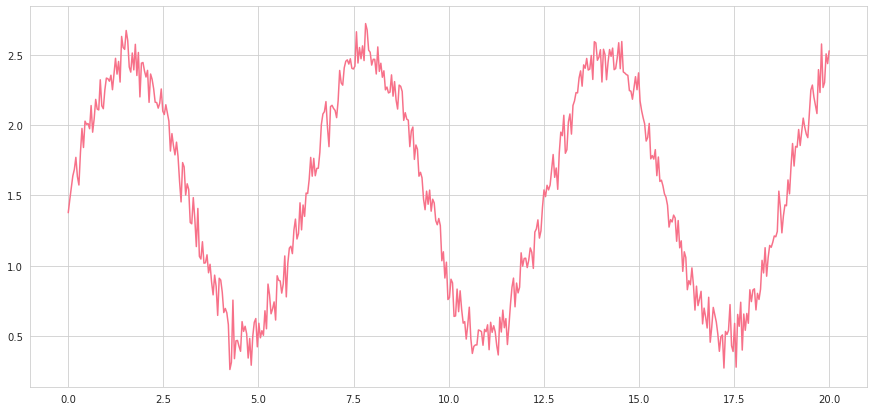
With a few styling choices, the plot looks presentable. However, there is one issue: by default, Seaborn does not begin at a zero baseline, and the numerical impact of the y-axis is lost. Assuming that the x and y variables are named as such, adding plt.fill_between(x,y,alpha=0.4) will turn the data into an area chart that more nicely begins at the base line and emphasizes the y-axis.

通過一些樣式選擇，該圖看起來很合適。 但是，存在一個問題：默認情況下，Seaborn并不是從零基線開始的，并且y軸的數值影響會丟失。 假設x和y變量是這樣命名的，則添加plt.fill_between(x,y,alpha=0.4)會將數據轉換為面積圖，該圖從基線開始會更好，并強調y軸。

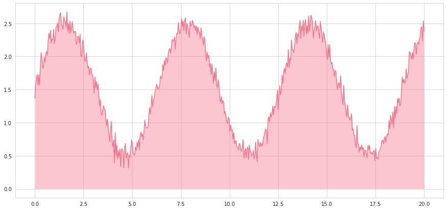
Note that this line is added in conjunction with the original lineplot, sns.lineplot(x,y), which provides the bolded line at the top. The alpha parameter, which appears in many seaborn plots as well, controls the transparency of the area (the less, the lighter). plt represents the matplotlib library. In some cases, using area may not be suitable.

請注意，這條線是與原始線圖sns.lineplot(x,y) ，它在頂部提供了粗體線。 alpha參數(也出現在許多海洋圖中)控制著區域的透明度(越少越亮)。 plt代表matplotlib庫。 在某些情況下，使用區域可能不合適。

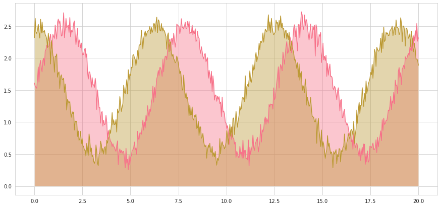
When multiple area plots are used, it can emphasize overlapping and intersections of the lines, although, again, it may not be appropriate for the visualization context.

當使用多個區域圖時，它可以強調線的重疊和相交，盡管同樣，它可能不適用于可視化上下文。

線圖到堆疊區域圖 (Line plot to stacked area plot)

Sometimes, the relationship between lines requires that the area plots be stacked on top of each other. This is easy to do with matplotlib stackplot: plt.stackplot(x,y,alpha=0.4). In this case, colors were manually specified through colors=[], which takes in a list of color names or hex codes.

有時，線之間的關系要求面積圖彼此堆疊。 使用matplotlib stackplot很容易做到： plt.stackplot(x,y,alpha=0.4) 。 在這種情況下，顏色是通過colors=[]手動指定的，它接受顏色名稱或十六進制代碼的列表。

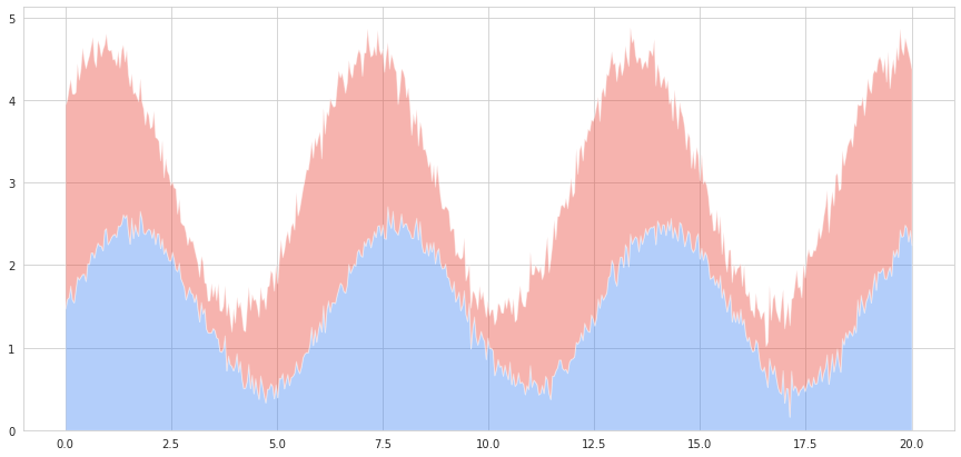
Note that y is a list of y1 and y2, which represent the noisy sine and cosine waves. These are stacked on top of each other in the area representation, and can heighten understanding of the relative distance between two area plots.

請注意， y是y1和y2的列表，它們代表有噪聲的正弦波和余弦波。 它們在區域表示中彼此堆疊，可以加深對兩個區域圖之間相對距離的理解。

刪除討厭的傳說 (Remove pesky legends)

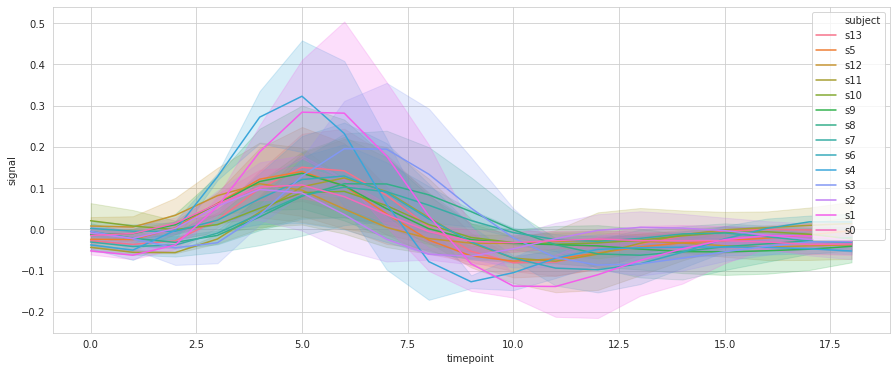
Seaborn often uses legends by default when the hue parameter is called to draw multiple of the same plot, differing by the column specified as the hue. These legends, while sometimes helpful, often cover up important parts of the plot and contain information that could be better expressed elsewhere (perhaps in a caption).

默認情況下，在調用hue參數繪制同一圖的倍數時，Seaborn通常默認使用圖例，不同之處在于指定為hue的列。 這些圖例雖然有時會有所幫助，但通常會掩蓋劇情中的重要部分，并包含可以在其他地方更好地表達的信息(也許在標題中)。

For example, consider the following medical dataset, which contains signals from various subjects. In this case, we want to use multiple line plots to visualize the general trend and range across different patients by setting the subject column as the hue (yes, putting this many lines is known as a ‘spaghetti chart’ and is generally not advised). One can see how the default labels are a) not ordered, b) so long that it obstructs part of the chart, and c) not the point of the visualization.

例如，考慮以下醫療數據集，其中包含來自各個受試者的信號。 在這種情況下，我們希望使用多個折線圖，通過將subject列設置為hue來可視化不同患者的總體趨勢和范圍(是的，放置這么多折線被稱為“意大利面條圖”，通常不建議這樣做) 。 可以看到默認標簽是如何排列的：a)沒有排序，b)太長以致于它阻礙了圖表的一部分，并且c)沒有可視化的要點。

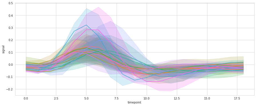
This can be done by setting the plot equal to a variable (commonly g), like such: g=sns.lineplot(x=…, y=…, hue=…). Then, by accessing the plot object’s legend attributes, we can remove it: g.legend_.remove(). If you are working with a grid object like PairGrid or FacetGrid, use g._legend.remove().

這可以通過將繪圖設置為等于變量(通常為g )來完成，例如： g=sns.lineplot(x=…, y=…, hue=…) 。 然后，通過訪問繪圖對象的圖例屬性，可以將其刪除： g.legend_.remove() 。 如果您正在使用諸如PairGrid或FacetGrid之類的網格對象，請使用g._legend.remove() 。

手動X和Y軸基線 (Manual x and y axis baselines)

Seaborn does not draw the x and y axis lines by default, but the axes are important for understanding not only the shape of the data but where they stand in relation to the coordinate system.

Seaborn默認情況下不會繪制x和y軸線，但是這些軸不僅對于理解數據的形狀而且對于理解其相對于坐標系的位置非常重要。

Matplotlib provides a simple way to add the x-axis by simply adding g.axhline(0), where g is the grid object and 0 represents the y-axis value at which the horizontal line is placed. Additionally, one can specify color (in this case color=’black’) and alpha (transparency, in this case alpha=0.5). linestyle is a parameter used to create dotted lines by being set to ‘--’.

Matplotlib提供了一種簡單的方法，只需添加g.axhline(0)即可添加x軸，其中g是網格對象，0表示放置水平線的y軸值。 另外，可以指定color (在這種情況下為color='black' )和alpha (透明度，在這種情況下為alpha=0.5 )。 linestyle是用于通過將其設置為'--'來創建虛線的參數。

Additionally, vertical lines can be added through g.axvline(0).

另外，可以通過g.axvline(0)添加垂直線。

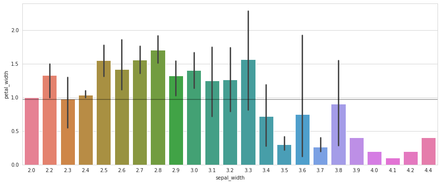
You can also use axhline to display averages or benchmarks for, say, bar plots. For example, say that we want to show the plants that were able to meet the 0.98 petal_width benchmark based on sepal_width.

您還可以使用axhline顯示axhline平均值或基準。 例如，假設我們要顯示能夠滿足基于sepal_width petal_width基準的sepal_width 。

對數刻度 (Logarithmic Scales)

Logarithmic scales are used because they can show a percent change. In many scenarios, this is exactly what is necessary — after all, an increase of $1000 for a business that normally earns $300 is not the same as an increase of $1000 for a megacorporation that earns billions. Instead of needing to calculate percentages in the data, matplotlib can convert scales to logarithmic.

使用對數刻度，因為它們可以顯示百分比變化。 在許多情況下，這正是必要的條件—畢竟，通常賺取300美元的企業增加1000美元，與賺取數十億美元的大型企業增加1000美元并不相同。 matplotlib無需計算數據中的百分比，而是可以將比例轉換為對數。

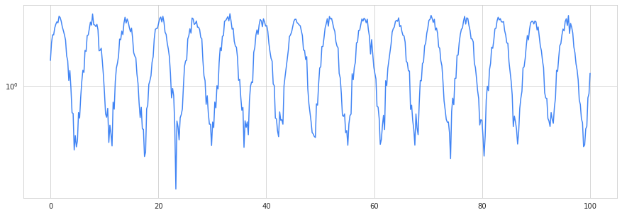
As with many matplotlib features, logarithmic scales operate on the ax of a standard figure created with fig, ax = plt.subplots(figsize=(x,y)). Then, a logarithmic x-scale is as simple as ax.set_xscale(‘log’):

與許多matplotlib功能一樣，對數刻度在用fig, ax = plt.subplots(figsize=(x,y))創建的標準圖形的fig, ax = plt.subplots(figsize=(x,y)) 。 然后，對數x ax.set_xscale('log')與ax.set_xscale('log')一樣簡單：

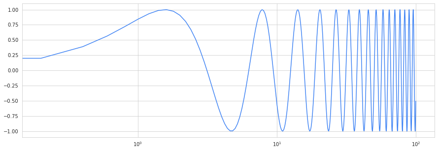
A logarithmic y-scale, which is more commonly used, can be done with ax.setyscale(‘log’):

可以使用ax.setyscale('log')完成更常用的對數y ax.setyscale('log') ：

榮譽獎 (Honorable mentions)

• Invest in a good default palette. Color is one of the most important aspects of a visualization: it ties it together and expressed a theme. You can choose and set one of Seaborn’s many great palettes with sns.set_palette(name). Check out demonstrations and tips to choosing palettes here.

  投資一個好的默認調色板。 顏色是可視化的最重要方面之一：顏色將其綁在一起并表達了主題。 您可以使用sns.set_palette(name)選擇并設置Seaborn的眾多出色調色板sns.set_palette(name) 。 在此處查看演示和選擇調色板的提示。

• You can add grids and change the background color with sns.set_style(name), where name can be white (default), whitegrid, dark, or darkgrid.

  您可以使用sns.set_style(name)添加網格并更改背景顏色，其中name可以是white (默認)， whitegrid ， dark或darkgrid 。

• Did you know that matplotlib and seaborn can process LaTeX, the beautiful mathematical formatting language? You can use it in your x/y axis labels, titles, legends, and more by enclosing LaTeX expressions within dollar signs $expression$.

  您是否知道matplotlib和seaborn可以處理LaTeX(一種漂亮的數學格式化語言) ？ 通過將LaTeX表達式包含在美元符號$expression$ ，可以在x / y軸標簽，標題，圖例等中使用它。

• Explore different linestyles, annotation sizes, and fonts. Matplotlib is full of them, if only you have the will to explore its documentation pages.
  探索不同的線型，注釋大小和字體。 Matplotlib充滿了它們，只要您愿意探索它的文檔頁面。

• Most plots have additional parameters, such as error bars for bar plots, thickness, dotted lines, and transparency for line plots. Taking some time to visit the documentation pages and peering through all the available parameters can take only a minute but has the potential to bring your visualization to top-notch aesthetic and informational value.

  大多數圖都有其他參數，例如條形圖的誤差線，厚度，虛線和線圖的透明度。 花一些時間訪問文檔頁面并瀏覽所有可用參數僅需一分鐘，但有可能使您的可視化達到一流的美學和信息價值。

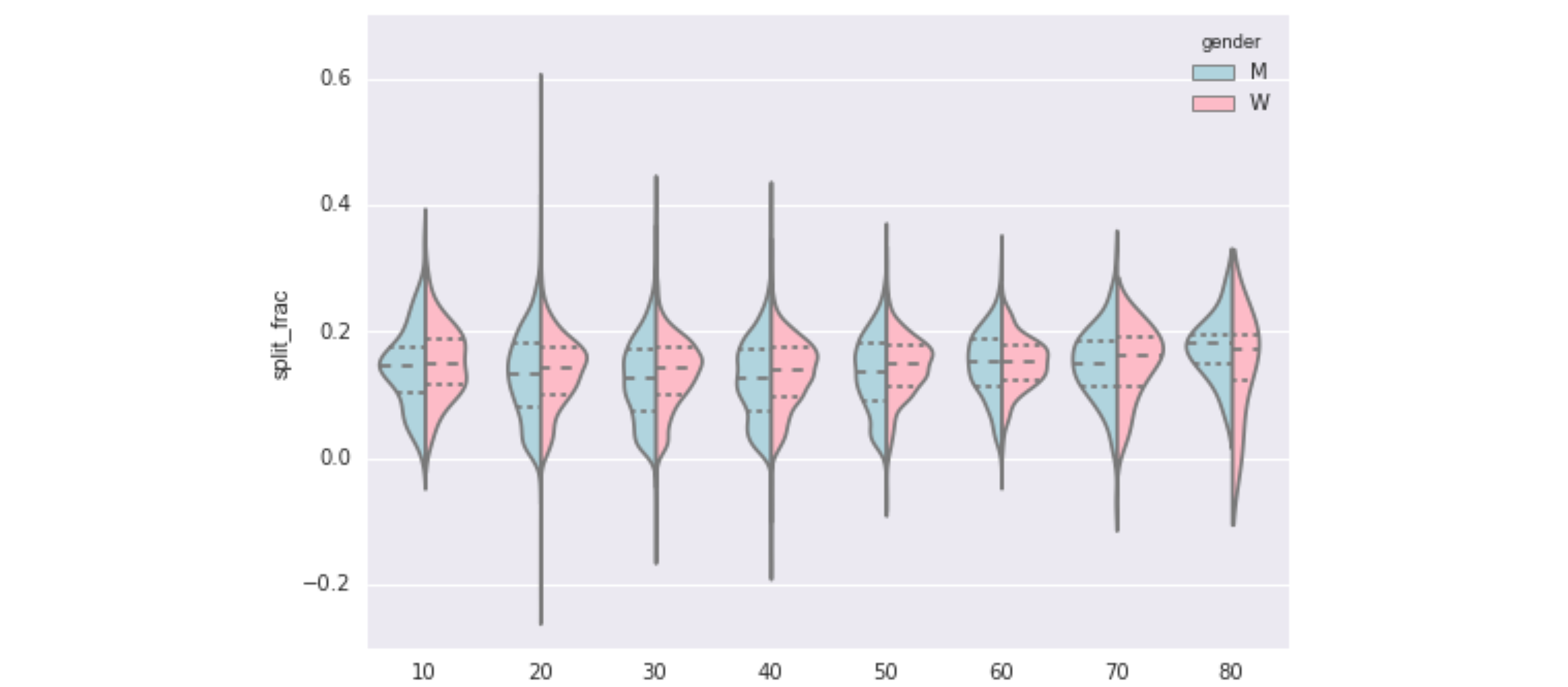
  For example, adding the parameter

  例如，添加參數

  inner=’quartile’ in a violinplot draws the first, second, and third quartiles of a distribution in dotted lines. Two words for immense informational gain — I’d say that’s a good deal!

  小提琴圖中的inner='quartile' quartile inner='quartile'用虛線繪制分布的第一，第二和第三四分位數。 兩個詞可帶來巨大的信息收益-我說這很劃算！

附加閱讀 (Additional Reading)

All charts created by author.

所有圖表由作者創建。