When I started on my journey to learn data science, I read through multiple articles that stressed the importance of understanding your data. It didn’t make sense to me. I was naive enough to think that we are handed over data which we push through an algorithm and hand over the results.

當我開始學習數據科學的旅程時，我通讀了多篇文章，其中強調了理解您的數據的重要性。 對我來說這沒有意義。 我很天真，以為我們已經交出了我們通過算法推送并交出結果的數據。

Yes, I wasn’t exactly the brightest. But I’ve learned my lesson and today I want to impart what I picked from my sleepless nights trying to figure out my data. I am going to use the R language to demonstrate EDA.

是的，我并不是最聰明的人。 但是我已經吸取了教訓，今天我想講講我從不眠之夜中挑選出的東西，以弄清楚我的數據。 我將使用R語言來演示EDA。

WHY R?

為什么R？

Because it was built from the get-go keeping data science in mind. It’s easy to pick up and get your hands dirty and doesn’t have a steep learning curve, *cough* Assembly *cough*.

因為它是從一開始就牢記數據科學而構建的。 它很容易拿起并弄臟您的手，沒有陡峭的學習曲線，*咳嗽* 組裝 *咳嗽*。

Before I start, This article is a guide for people classified under the tag of ‘Data Science infants.’ I believe both Python and R are great languages, and what matters most is the Story you tell from your data.

在開始之前，本文是針對歸類為“數據科學嬰兒”標簽的人們的指南。 我相信Python和R都是很棒的語言，最重要的是您從數據中講述的故事。

為什么使用此數據集？ (Why this dataset?)

Well, it’s where I think most of the aspiring data scientists would start. This data set is a good starting place to heat your engines to start thinking like a data scientist at the same time being a novice-friendly helps you breeze through the exercise.

好吧，這是我認為大多數有抱負的數據科學家都會從那里開始的地方。 該數據集是加熱引擎以像數據科學家一樣開始思考的良好起點，同時對新手友好，可以幫助您輕而易舉地完成練習。

我們如何處理這些數據？ (How do we approach this data?)

• Will this variable help use predict house prices?
  這個變量是否有助于預測房價？
• Is there a correlation between these variables?
  這些變量之間有相關性嗎？
• Univariate Analysis
  單變量分析
• Multivariate Analysis
  多元分析
• A bit of Data Cleaning
  一點數據清理
• Conclude with proving the relevance of our selected variables.
  最后證明我們選擇的變量的相關性。

Best of luck on your journey to master Data Science!

在掌握數據科學的過程中祝您好運！

Now, we start with importing packages, I’ll explain why these packages are present along the way…

現在，我們從導入程序包開始，我將解釋為什么這些程序包一直存在...

easypackages::libraries("dplyr", "ggplot2", "tidyr", "corrplot", "corrr", "magrittr",   "e1071","ggplot2","RColorBrewer", "viridis")
options(scipen = 5)      #To force R to not use scientfic notationdataset <- read.csv("train.csv")
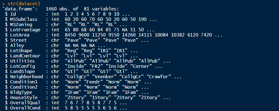
str(dataset)

Here, in the above snippet, we use scipen to avoid scientific notation. We import our data and use the str() function to get the gist of the selection of variables that the dataset offers and the respective data type.

在此，在上面的代碼段中，我們使用scipen來避免科學計數法。 我們導入數據并使用str()函數來獲取數據集提供的變量以及相應數據類型的選擇依據。

The variable SalePrice is the dependent variable which we are going to base all our assumptions and hypothesis around. So it’s good to first understand more about this variable. For this, we’ll use a Histogram and fetch a frequency distribution to get a visual understanding of the variable. You’d notice there’s another function i.e. summary() which is essentially used to for the same purpose but without any form of visualization. With experience, you’ll be able to understand and interpret this form of information better.

變量SalePrice是因變量，我們將基于其所有假設和假設。 因此，最好先了解更多有關此變量的信息。 為此，我們將使用直方圖并獲取頻率分布以直觀了解變量。 您會注意到還有另一個函數，即summary()，該函數本質上用于相同的目的，但沒有任何形式的可視化。 憑借經驗，您將能夠更好地理解和解釋這種形式的信息。

ggplot(dataset, aes(x=SalePrice)) + 
  theme_bw()+
  geom_histogram(aes(y=..density..),color = 'black', fill = 'white', binwidth = 50000)+
  geom_density(alpha=.2, fill='blue') +
  labs(title = "Sales Price Density", x="Price", y="Density")summary(dataset$SalePrice)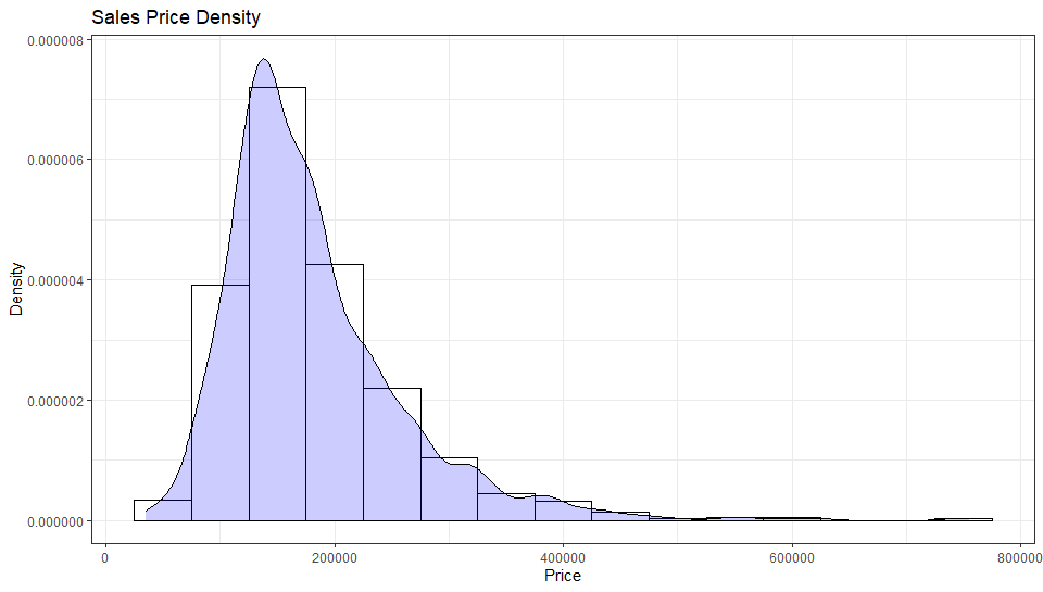

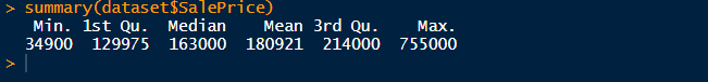
So it is pretty evident that you’ll find many properties in the sub $200,000 range. There are properties over $600,000 and we can try to understand why is it so and what makes these homes so ridiculously expensive. That can be another fun exercise…

因此，很明顯，您會找到許多價格在20萬美元以下的物業。 有超過60萬美元的物業，我們可以試著理解為什么會這樣，以及是什么使這些房屋如此昂貴。 那可能是另一個有趣的練習……

在確定要購買的房屋的價格時，您認為哪些變量影響最大？ (Which variables do you think are most influential when deciding a price for a house you are looking to buy?)

Now that we have a basic idea about SalePrice we will try to visualize this variable in terms of some other variable. Please note that it is very important to understand what type of variable you are working with. I would like you to refer to this amazing article which covers this topic in more detail here.

現在，我們對SalePrice有了基本的了解，我們將嘗試根據其他變量來形象化此變量。 請注意，了解要使用的變量類型非常重要。 我想你指的這個驚人的物品，其更為詳細地介紹這個主題在這里 。

Moving on, We will be dealing with two kinds of variables.

繼續，我們將處理兩種變量。

• Categorical Variable
  分類變量
• Numeric Variable
  數值變量

Looking back at our dataset we can discern between these variables. For starters, we run a coarse comb across the dataset and guess pick some variables which have the highest chance of being relevant. Note that these are just assumptions and we are exploring this dataset to understand this. The variables I selected are:

回顧我們的數據集，我們可以區分這些變量。 首先，我們對數據集進行粗梳，并猜測選擇一些具有最大相關性的變量。 請注意，這些只是假設，我們正在探索此數據集以理解這一點。 我選擇的變量是：

• GrLivArea
  GrLivArea
• TotalBsmtSF
  TotalBsmtSF
• YearBuilt
  建立年份
• OverallQual
  綜合素質

So which ones are Quantitive and which ones are Qualitative out of the lot? If you look closely the OveralQual and YearBuilt variable then you will notice that these variables can never be Quantitative. Year and Quality both are categorical by nature of this data however, R doesn’t know that. For that, we use factor() function to convert a numerical variable to categorical so R can interpret the data better.

那么，哪些是定量的，哪些是定性的呢？ 如果仔細查看OveralQual和YearBuilt變量，您會注意到這些變量永遠不會是定量的。 年和質量都是根據此數據的性質分類的，但是R不知道。 為此，我們使用factor()函數將數值變量轉換為分類變量，以便R可以更好地解釋數據。

dataset$YearBuilt <- factor(dataset$YearBuilt)
dataset$OverallQual <- factor(dataset$OverallQual)

Now when we run str() on our dataset we will see both YearBuilt and OverallQual as factor variables.

現在，當我們在數據集上運行str()時 ，我們會將YearBuilt和TotalQual都視為因子變量。

We can now start plotting our variables.

現在，我們可以開始繪制變量。

關系非常復雜 (Relationships are (NOT) so complicated)

Taking YearBuilt as our first candidate we start plotting.

以YearBuilt作為我們的第一個候選人，我們開始繪圖。

ggplot(dataset, aes(y=SalePrice, x=YearBuilt, group=YearBuilt, fill=YearBuilt)) +
  theme_bw()+
  geom_boxplot(outlier.colour="red", outlier.shape=8, outlier.size=1)+
  theme(legend.position="none")+
  scale_fill_viridis(discrete = TRUE) +
  theme(axis.text.x = element_text(angle = 90))+
  labs(title = "Year Built vs. Sale Price", x="Year", y="Price")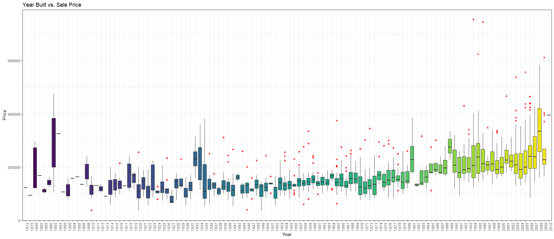

Old houses sell for less as compared to a recently built house. And as for OverallQual,

與最近建造的房屋相比，舊房屋的售價更低。 至于TotalQuality ，

ggplot(dataset, aes(y=SalePrice, x=OverallQual, group=OverallQual,fill=OverallQual)) +
  geom_boxplot(alpha=0.3)+
  theme(legend.position="none")+
  scale_fill_viridis(discrete = TRUE, option="B") +
  labs(title = "Overall Quality vs. Sale Price", x="Quality", y="Price")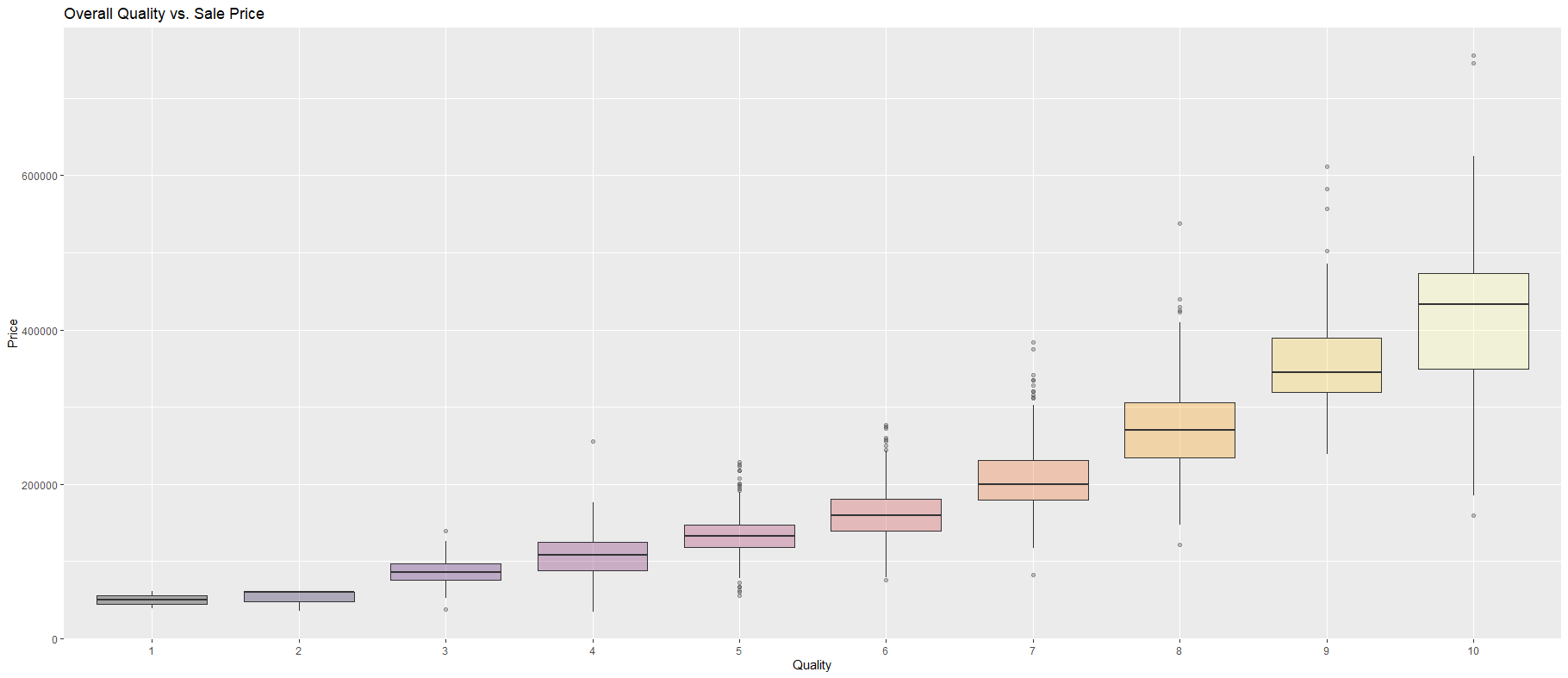

This was expected since you’d naturally pay more for the house which is of better quality. You won’t want your foot to break through the floorboard, will you? Now that the qualitative variables are out of the way we can focus on the numeric variables. The very first candidate we have here is GrLivArea.

這是預料之中的，因為您自然會為質量更好的房子付出更多。 您不希望您的腳摔破地板，對嗎？ 現在，定性變量已不復存在，我們可以將重點放在數字變量上。 我們在這里擁有的第一個候選人是GrLivArea 。

ggplot(dataset, aes(x=SalePrice, y=GrLivArea)) +
  theme_bw()+
  geom_point(colour="Blue", alpha=0.3)+
  theme(legend.position='none')+
  labs(title = "General Living Area vs. Sale Price", x="Price", y="Area")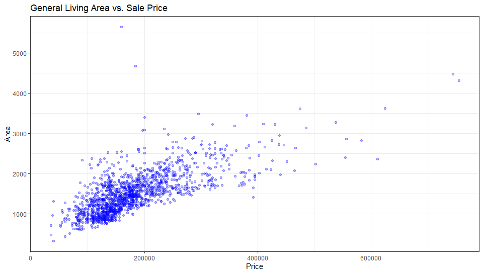

I would be lying if I said I didn’t expect this. The very first instinct of a customer is to check the area of rooms. And I think the result will be the same for TotalBsmtASF. Let’s see…

如果我說我沒想到這一點，我會撒謊。 顧客的本能是檢查房間的面積。 而且我認為結果與TotalBsmtASF相同。 讓我們來看看…

ggplot(dataset, aes(x=SalePrice, y=TotalBsmtSF)) +
  theme_bw()+
  geom_point(colour="Blue", alpha=0.3)+
  theme(legend.position='none')+
  labs(title = "Total Basement Area vs. Sale Price", x="Price", y="Area")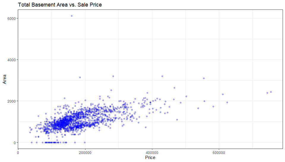

那么我們能說些什么呢？ (So what can we say about our cherry-picked variables?)

GrLivArea and TotalBsmtSF both were found to be in a linear relation with SalePrice. As for the categorical variables, we can say with confidence that the two variable which we picked were related to SalePrice with confidence.

發現GrLivArea和TotalBsmtSF都與SalePrice呈線性關系。 至于分類變量，我們可以放心地說，我們選擇的兩個變量與SalePrice有信心。

But these are not the only variables and there’s more to than what meets the eye. So to tread over these many variables we’ll take help from a correlation matrix to see how each variable correlate to get a better insight.

但是，這些并不是唯一的變量，還有比眼球更重要的事情。 因此，要遍歷這些變量，我們將從關聯矩陣中獲取幫助，以了解每個變量之間的關聯方式，從而獲得更好的見解。

相關圖的時間 (Time for Correlation Plots)

So what is Correlation?

那么什么是相關性？

Correlation is a measure of how well two variables are related to each other. There are positive as well as negative correlation.

相關性是兩個變量之間相關程度的度量。 正相關和負相關。

If you want to read more on Correlation then take a look at this article. So let’s create a basic Correlation Matrix.

如果您想閱讀有關Correlation的更多信息，請閱讀本文 。 因此，讓我們創建一個基本的“相關矩陣”。

M <- cor(dataset)
M <- dataset %>% mutate_if(is.character, as.factor)
M <- M %>% mutate_if(is.factor, as.numeric)
M <- cor(M)mat1 <- data.matrix(M)
print(M)#plotting the correlation matrix
corrplot(M, method = "color", tl.col = 'black', is.corr=FALSE)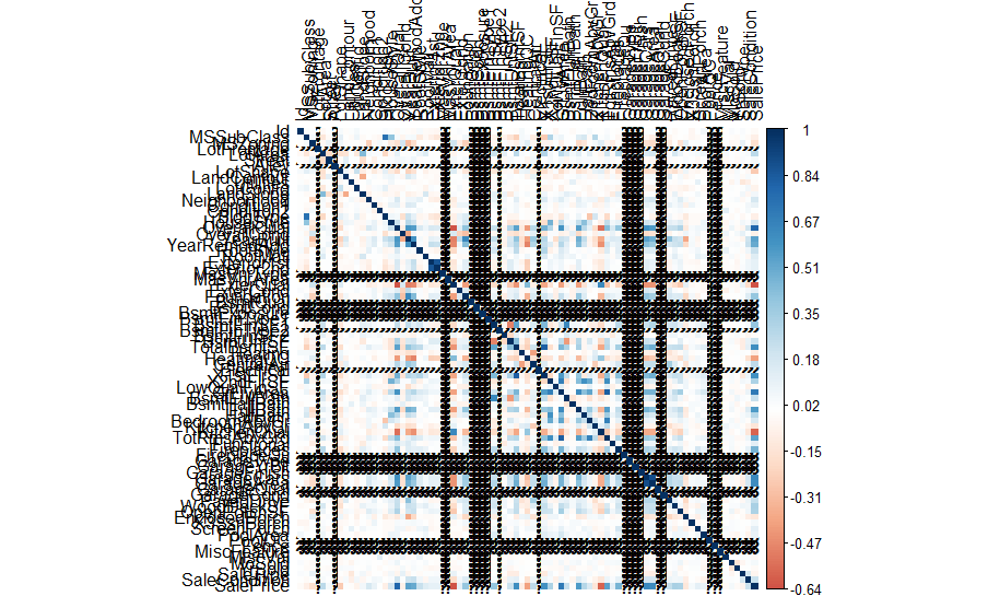

請不要關閉此標簽。 我保證會好起來的。 (Please don’t close this tab. I promise it gets better.)

But worry not because now we’re going to get our hands dirty and make this plot interpretable and tidy.

但是不用擔心，因為現在我們要動手做，使這段情節變得可解釋和整潔。

M[lower.tri(M,diag=TRUE)] <- NA                   #remove coeff - 1 and duplicates
M[M == 1] <- NAM <- as.data.frame(as.table(M))                   #turn into a 3-column table
M <- na.omit(M)                                   #remove the NA values from aboveM <- subset(M, abs(Freq) > 0.5)              #select significant values, in this case, 0.5
M <- M[order(-abs(M$Freq)),]                                  #sort by highest correlationmtx_corr <- reshape2::acast(M, Var1~Var2, value.var="Freq")    #turn M back into matrix 
corrplot(mtx_corr, is.corr=TRUE, tl.col="black", na.label=" ") #plot correlations visually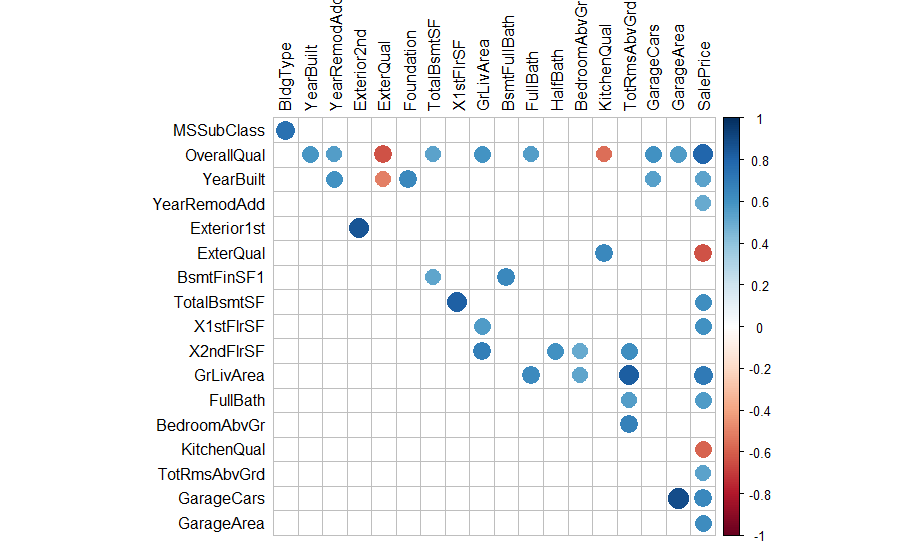

現在，這看起來更好而且可讀。 (Now, this looks much better and readable.)

Looking at our plot we can see numerous other variables that are highly correlated with SalePrice. We pick these variables and then create a new dataframe by only including these select variables.

查看我們的圖，我們可以看到許多與SalePrice高度相關的其他變量。 我們選擇這些變量，然后僅通過包含這些選擇變量來創建新的數據框。

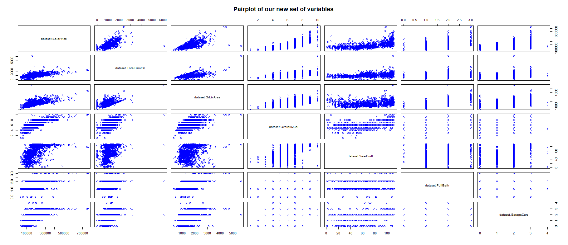
Now that we have our suspect variables we can use a PairPlot to visualize all these variables in conjunction with each other.

現在我們有了可疑變量，我們可以使用PairPlot將所有這些變量相互可視化。

newData <- data.frame(dataset$SalePrice, dataset$TotalBsmtSF, 
                      dataset$GrLivArea, dataset$OverallQual, 
                      dataset$YearBuilt, dataset$FullBath, 
                      dataset$GarageCars )pairs(newData[1:7], 
      col="blue",
      main = "Pairplot of our new set of variables"         
)

在處理數據時，請清理數據 (While you’re at it, clean your data)

We should remove some useless variables which we are sure of not being of any use. Don’t apply changes to the original dataset though. Always create a new copy in case you remove something you shouldn’t have.

我們應該刪除一些肯定不會有任何用處的無用變量。 但是不要將更改應用于原始數據集。 始終創建一個新副本，以防萬一您刪除了不該擁有的內容。

clean_data <- dataset[,!grepl("^Bsmt",names(dataset))]      #remove BSMTx variablesdrops <- c("clean_data$PoolQC", "clean_data$PoolArea", 
               "clean_data$FullBath", "clean_data$HalfBath")
               
clean_data <- clean_data[ , !(names(clean_data) %in% drops)]#The variables in 'drops'are removed.

單變量分析 (Univariate Analysis)

Taking a look back at our old friend, SalePrice, we see some extremely expensive houses. We haven’t delved into why is that so. Although we do know that these extremely pricey houses don’t follow the pattern which other house prices are following. The reason for such high prices could be justified but for the sake of our analysis, we have to drop them. Such records are called Outliers.

回顧一下我們的老朋友SalePrice ，我們看到了一些極其昂貴的房子。 我們還沒有深入研究為什么會這樣。 盡管我們確實知道這些極其昂貴的房子沒有遵循其他房價正在遵循的模式。 如此高的價格的原因是有道理的，但出于我們的分析考慮，我們必須將其降低。 這樣的記錄稱為離群值。

Simple way to understand Outliers is to think of them as that one guy (or more) in your group who likes to eat noodles with a spoon instead of a fork.

理解離群值的簡單方法是將其視為小組中的一個(或多個)喜歡用勺子而不是叉子吃面條的人。

So first, we catch these outliers and then remove them from our dataset if need be. Let’s start with the catching part.

因此，首先，我們捕獲這些離群值，然后根據需要將其從數據集中刪除。 讓我們從捕捉部分開始。

#Univariate Analysisclean_data$price_norm <- scale(clean_data$SalePrice)    #normalizing the price variablesummary(clean_data$price_norm)plot1 <- ggplot(clean_data, aes(x=factor(1), y=price_norm)) +
  theme_bw()+
  geom_boxplot(width = 0.4, fill = "blue", alpha = 0.2)+
  geom_jitter( 
              width = 0.1, size = 1, aes(colour ="red"))+
  geom_hline(yintercept=6.5, linetype="dashed", color = "red")+
  theme(legend.position='none')+
  labs(title = "Hunt for Outliers", x=NULL, y="Normalized Price")plot2 <- ggplot(clean_data, aes(x=price_norm)) + 
  theme_bw()+
  geom_histogram(color = 'black', fill = 'blue', alpha = 0.2)+
  geom_vline(xintercept=6.5, linetype="dashed", color = "red")+
  geom_density(aes(y=0.4*..count..), colour="red", adjust=4) +
  labs(title = "", x="Price", y="Count")grid.arrange(plot1, plot2, ncol=2)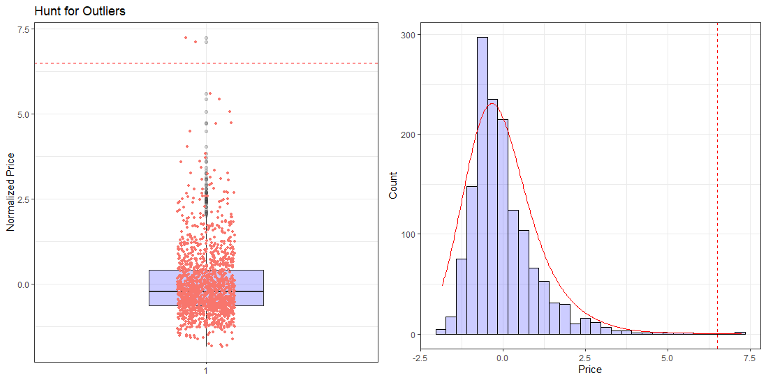

The very first thing I did here was normalize SalePrice so that it’s more interpretable and it’s easier to bottom down on these outliers. The normalized SalePrice has Mean= 0 and SD= 1. Running a quick ‘summary()’ on this new variable price_norm give us this…

我在這里所做的第一件事就是對SalePrice進行規范化，以使其更易于解釋，并且更容易查明這些異常值。 歸一化的SalePrice的均值= 0 ， SD = 1 。 在這個新變量price_norm上運行一個快速的“ summary()” ，可以給我們這個…

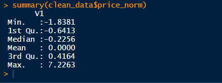
So now we know for sure that there ARE outliers present here. But do we really need to get rid of them? From the previous scatterplots we can say that these outliers are still following along with the trend and don’t need purging yet. Deciding what to do with outliers can be quite complex at times. You can read more on outliers here.

因此，現在我們可以肯定地知道這里有異常值。 但是我們真的需要擺脫它們嗎？ 從以前的散點圖可以看出，這些離群值仍在跟隨趨勢，并且不需要清除。 決定如何處理異常值有時可能非常復雜。 您可以在這里有關離群值的信息 。

雙變量分析 (Bi-Variate Analysis)

Bivariate analysis is the simultaneous analysis of two variables (attributes). It explores the concept of a relationship between two variables, whether there exists an association and the strength of this association, or whether there are differences between two variables and the significance of these differences. There are three types of bivariate analysis.

雙變量分析是對兩個變量(屬性)的同時分析。 它探討了兩個變量之間關系的概念，是否存在關聯和這種關聯的強度，或者兩個變量之間是否存在差異以及這些差異的重要性。 雙變量分析有三種類型。

• Numerical & Numerical
  數值與數值
• Categorical & Categorical
  分類和分類
• Numerical & Categorical
  數值和分類

The very first set of variables we will analyze here are SalePrice and GrLivArea. Both variables are Numerical so using a Scatter Plot is a good idea!

我們將在此處分析的第一組變量是SalePrice和GrLivArea 。 這兩個變量都是數值變量，因此使用散點圖是個好主意！

ggplot(clean_data, aes(y=SalePrice, x=GrLivArea)) +
  theme_bw()+
  geom_point(aes(color = SalePrice), alpha=1)+
  scale_color_gradientn(colors = c("#00AFBB", "#E7B800", "#FC4E07")) +
  labs(title = "General Living Area vs. Sale Price", y="Price", x="Area")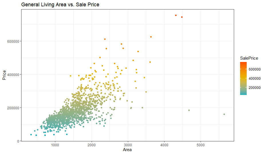

Immediately, we notice that 2 houses don’t follow the linear trend and affect both our results and assumptions. These are our outliers. Since our results in future are prone to be affected negatively by these outliers, we will remove them.

立刻，我們注意到有2所房屋沒有遵循線性趨勢，并且影響了我們的結果和假設。 這些是我們的異常值。 由于我們未來的結果很容易受到這些異常值的負面影響，因此我們將其刪除。

clean_data <- clean_data[!(clean_data$GrLivArea > 4000),]   #remove outliersggplot(clean_data, aes(y=SalePrice, x=GrLivArea)) +
  theme_bw()+
  geom_point(aes(color = SalePrice), alpha=1)+
  scale_color_gradientn(colors = c("#00AFBB", "#E7B800", "#FC4E07")) +
  labs(title = "General Living Area vs. Sale Price [Outlier Removed]", y="Price", x="Area")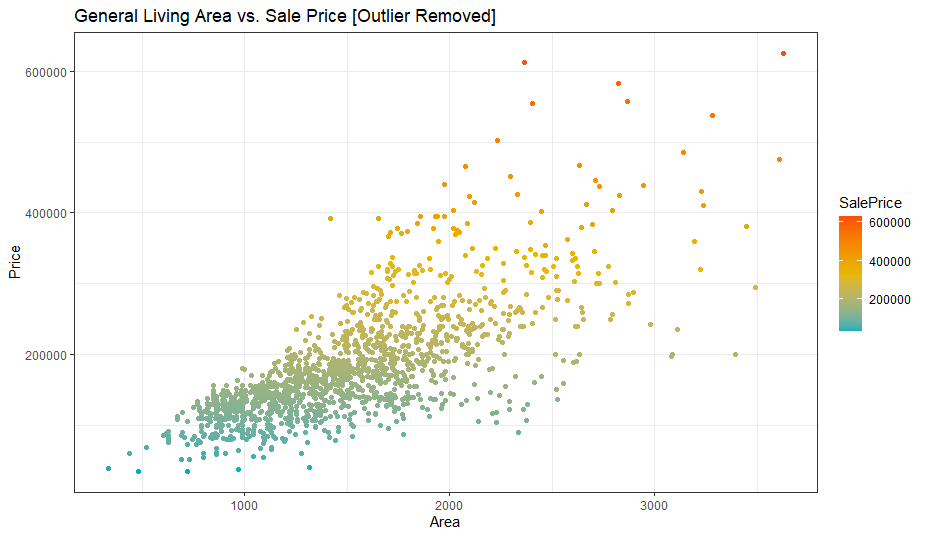

The outlier is removed and the x-scale is adjusted. Next set of variables which we will analyze are SalePrice and TotalBsmtSF.

移除異常值并調整x比例。 我們將分析的下一組變量是SalePrice和TotalBsmtSF 。

ggplot(clean_data, aes(y=SalePrice, x=TotalBsmtSF)) +
  theme_bw()+
  geom_point(aes(color = SalePrice), alpha=1)+
  scale_color_gradientn(colors = c("#00AFBB", "#E7B800", "#FC4E07")) +
  labs(title = "Total Basement Area vs. Sale Price", y="Price", x="Basement Area")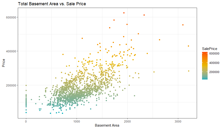

The observations here adhere to our assumptions and don’t need purging. If it ain’t broke, don’t fix it. I did mention that it is important to tread very carefully when working with outliers. You don’t get to remove them every time.

此處的觀察結果符合我們的假設，無需清除。 如果沒有損壞，請不要修復。 我確實提到過，在處理異常值時，請務必謹慎行事。 您不會每次都刪除它們。

是時候深入一點了 (Time to dig a bit deeper)

We based a ton of visualization around ‘SalePrice’ and other important variables, but what If I said that’s not enough? It’s not Because there’s more to dig out of this pit. There are 4 horsemen of Data Analysis which I believe people should remember.

我們圍繞“ SalePrice”和其他重要變量進行了大量可視化處理，但是如果我說那還不夠怎么辦？ 不是因為有更多東西需要挖掘。 我相信人們應該記住4位數據分析騎士。

• Normality: When we talk about normality what we mean is that the data should look like a normal distribution. This is important because a lot of statistic tests depend upon this (for example — t-statistics). First, we would check normality with just a single variable ‘SalePrice’(It’s usually better to start with a single variable). Though one shouldn’t assume that univariate normality would prove the existence of multivariate normality(which is comparatively more sought after), but it helps. Another thing to note is that in larger samples i.e. more than 200 samples, normality is not such an issue. However, A lot of problems can be avoided if we solve normality. That’s one of the reasons we are working with normality.

  正態性 ：當談論正態性時，我們的意思是數據看起來應該像正態分布。 這很重要，因為很多統計檢驗都依賴于此(例如t統計)。 首先，我們將僅使用單個變量“ SalePrice”(通常最好從單個變量開始)檢查正態性。 盡管不應該假設單變量正態性會證明多元正態性的存在(相對較受追捧)，但這很有幫助。 要注意的另一件事是，在較大的樣本(即200多個樣本)中，正態性不是問題。 但是，如果我們解決正態性，可以避免很多問題。 這就是我們進行正常工作的原因之一。

• Homoscedasticity: Homoscedasticity refers to the ‘assumption that one or more dependent variables exhibit equal levels of variance across the range of predictor variables’. If we want the error term to be the same across all values of the independent variable, then Homoscedasticity is to be checked.

  均方根性 ：均方根性是指“ 一個或多個因變量在預測變量范圍內表現出相等水平的方差的假設 ”。 如果我們希望誤差項在自變量的所有值上都相同，則將檢查同方差。

• Linearity: If you want to assess the linearity of your data then I believe scatter plots should be the first choice. Scatter plots can quickly show the linear relationship(if it exists). In the case where patterns are not linear, it would be worthwhile to explore data transformations. However, we need not check for this again since our previous plots have already proved the existence of a linear relationship.

  線性度 ：如果您想評估數據的線性度，那么我相信散點圖應該是首選。 散點圖可以快速顯示線性關系(如果存在)。 在模式不是線性的情況下，值得探索數據轉換。 但是，由于我們以前的曲線已經證明存在線性關系，因此我們無需再次檢查。

• Absence of correlated errors: When working with errors, if you notice a pattern where one error is correlated to another then there’s a relationship between these variables. For example, In a certain case, one positive error makes a negative error across the board then that would imply a relationship between errors. This phenomenon is more evident with time-sensitive data. If you do find yourself working with such data then try and add a variable that can explain your observations.

  缺少相關錯誤 ：處理錯誤時，如果您注意到一種模式，其中一個錯誤與另一個錯誤相關，則這些變量之間存在關聯。 例如，在某些情況下，一個正錯誤會在整個范圍內產生一個負錯誤，然后暗示錯誤之間的關系。 對于時間敏感的數據，這種現象更加明顯。 如果您發現自己正在使用此類數據，請嘗試添加一個可以解釋您的觀察結果的變量。

我認為我們應該開始做，而不是說 (I think we should start doing rather than saying)

Starting with SalePrice. Do keep an eye on the overall distribution of our variable.

從SalePrice開始。 請注意變量的總體分布。

plot3 <- ggplot(clean_data, aes(x=SalePrice)) + 
  theme_bw()+
  geom_density(fill="#69b3a2", color="#e9ecef", alpha=0.8)+
  geom_density(color="black", alpha=1, adjust = 5, lwd=1.2)+
  labs(title = "Sale Price Density", x="Price", y="Density")plot4 <- ggplot(clean_data, aes(sample=SalePrice))+
  theme_bw()+
  stat_qq(color="#69b3a2")+
  stat_qq_line(color="black",lwd=1, lty=2)+
  labs(title = "Probability Plot for SalePrice")grid.arrange(plot3, plot4, ncol=2)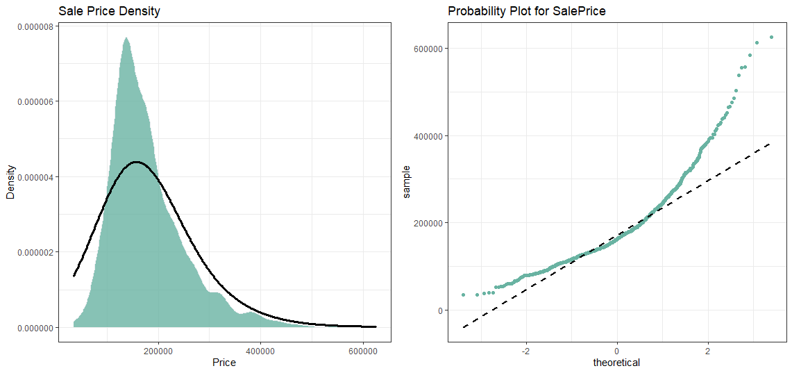

SalePrice is not normal! But we have another trick up our sleeves viz. log transformation. Now, one great thing about log transformation is that it can deal with skewed data and make it normal. So now it’s time to apply the log transformation over our variable.

促銷價不正常！ 但是，我們還有另外一個竅門。 日志轉換。 現在，關于日志轉換的一大優點是它可以處理偏斜的數據并使之正常。 因此，現在是時候將對數轉換應用于我們的變量了。

clean_data$log_price <- log(clean_data$SalePrice)plot5 <- ggplot(clean_data, aes(x=log_price)) + 
  theme_bw()+
  geom_density(fill="#69b3a2", color="#e9ecef", alpha=0.8)+
  geom_density(color="black", alpha=1, adjust = 5, lwd=1)+
  labs(title = "Sale Price Density [Log]", x="Price", y="Density")plot6 <- ggplot(clean_data, aes(sample=log_price))+
  theme_bw()+
  stat_qq(color="#69b3a2")+
  stat_qq_line(color="black",lwd=1, lty=2)+
  labs(title = "Probability Plot for SalePrice [Log]")grid.arrange(plot5, plot6, ncol=2)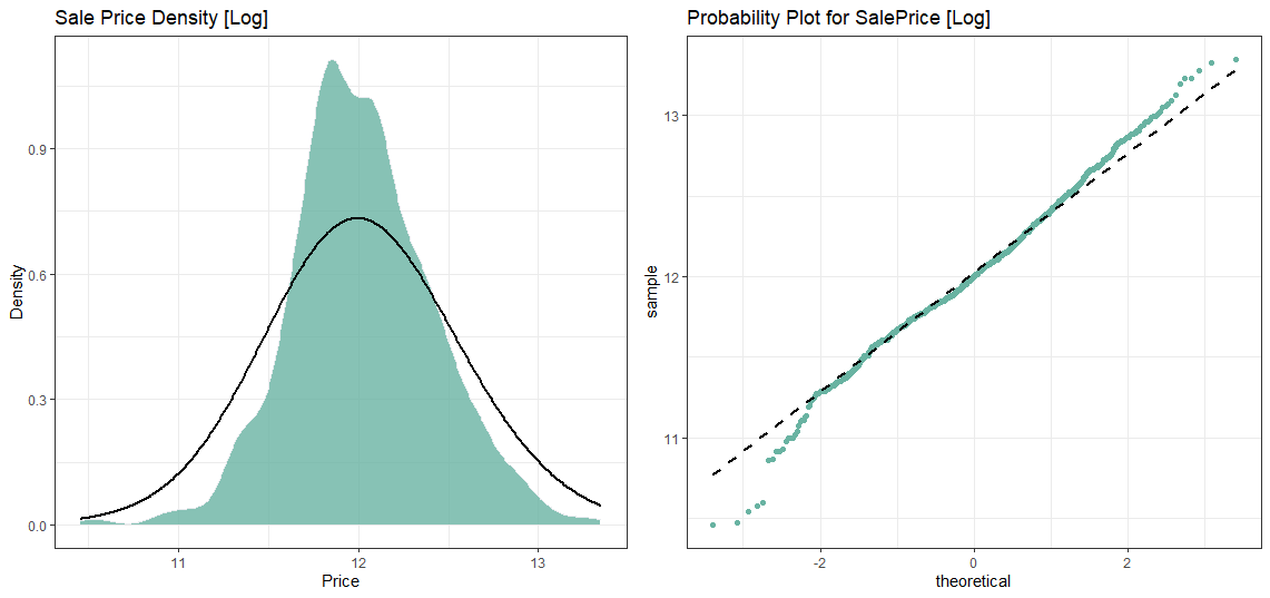

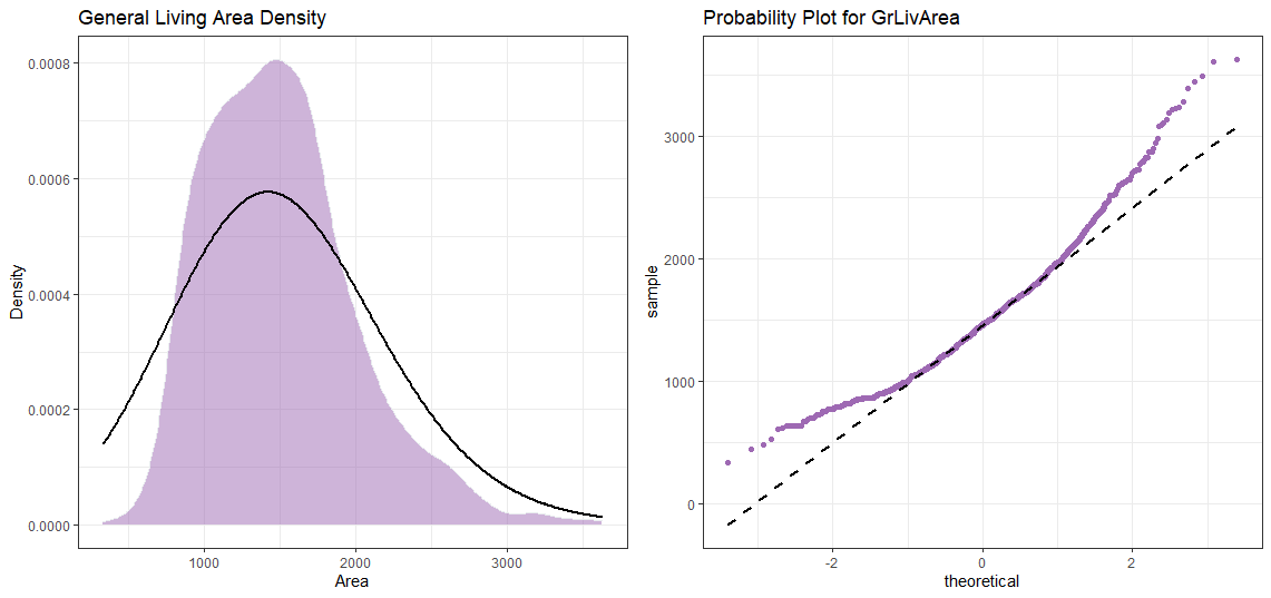
現在，使用其余的變量重復該過程。 (Now repeat the process with the rest of our variables.)

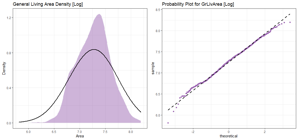
我們先和GrLivArea一起去 (We go with GrLivArea first)

日志轉換后 (After Log Transformation)

現在用于TotalBsmtSF (Now for TotalBsmtSF)

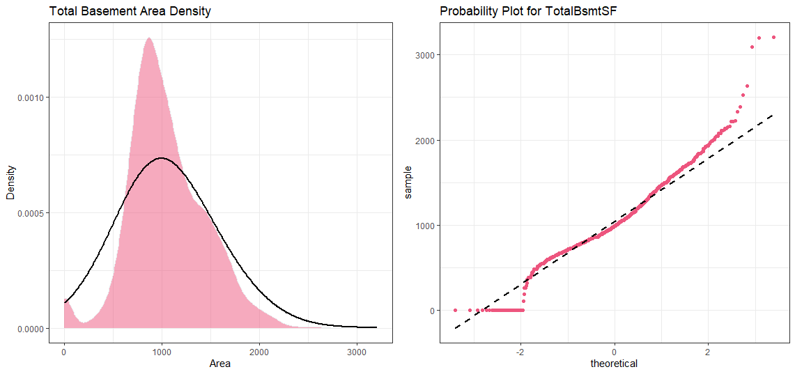
堅持，稍等！ 我們這里有一些有趣的東西。 (Hold On! We’ve got something interesting here.)

Looks like TotalBsmtSF has some zeroes. This doesn’t bode well with log transformation. We’ll have to do something about it. To apply a log transformation here, we’ll create a variable that can get the effect of having or not having a basement (binary variable). Then, we’ll do a log transformation to all the non-zero observations, ignoring those with value zero. This way we can transform data, without losing the effect of having or not the basement.

看起來TotalBsmtSF有一些零。 這對日志轉換不是一個好兆頭。 我們必須對此做些事情。 要在此處應用對數轉換，我們將創建一個變量，該變量可以具有或不具有地下室的效果(二進制變量)。 然后，我們將對所有非零觀測值進行對數轉換，而忽略值為零的觀測值。 這樣，我們可以轉換數據，而不會失去擁有或不擁有地下室的影響。

#The step where I create a new variable to dictate which row to transform and which to ignore
clean_data <- transform(clean_data, cat_bsmt = ifelse(TotalBsmtSF>0, 1, 0))#Now we can do log transformation
clean_data$totalbsmt_log <- log(clean_data$TotalBsmtSF)clean_data<-transform(clean_data,totalbsmt_log = ifelse(cat_bsmt == 1, log(TotalBsmtSF), 0 ))plot13 <- ggplot(clean_data, aes(x=totalbsmt_log)) + 
  theme_bw()+
  geom_density(fill="#ed557e", color="#e9ecef", alpha=0.5)+
  geom_density(color="black", alpha=1, adjust = 5, lwd=1)+
  labs(title = "Total Basement Area Density [transformed]", x="Area", y="Density")plot14 <- ggplot(clean_data, aes(sample=totalbsmt_log))+
  theme_bw()+
  stat_qq(color="#ed557e")+
  stat_qq_line(color="black",lwd=1, lty=2)+
  labs(title = "Probability Plot for TotalBsmtSF [transformed]")grid.arrange(plot13, plot14, ncol=2)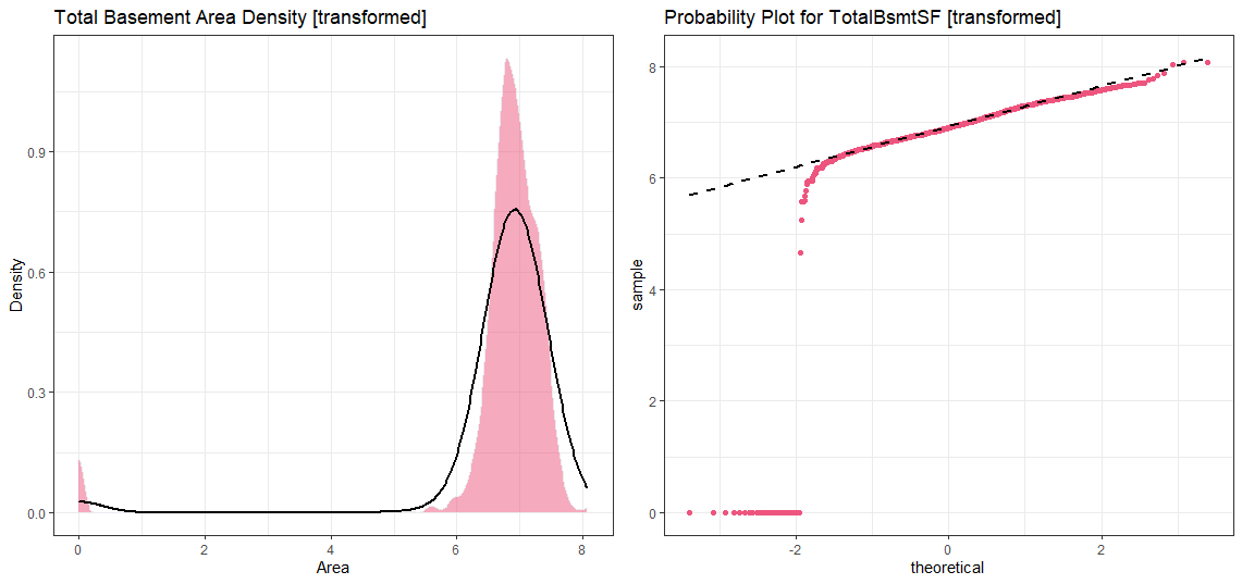

We can still see the ignored data points on the chart but hey, I can trust you with this, right?

我們仍然可以在圖表上看到被忽略的數據點，但是，我可以相信您，對嗎？

均方根性-等待我的拼寫正確嗎？ (Homoscedasticity — Wait is my spelling correct?)

The best way to look for homoscedasticity is to work try and visualize the variables using charts. A scatter plot should do the job. Notice the shape which the data forms when plotted. It could look like an equal dispersion which looks like a cone or it could very well look like a diamond where a large number of data points are spread around the centre.

尋找同質性的最佳方法是嘗試使用圖表直觀顯示變量。 散點圖可以完成這項工作。 注意繪制時數據形成的形狀。 它可能看起來像一個均勻的色散，看起來像一個圓錐形，或者看起來非常像一個菱形，其中大量數據點圍繞中心分布。

Starting with ‘SalePrice’ and ‘GrLivArea’…

從“ SalePrice”和“ GrLivArea”開始...

ggplot(clean_data, aes(x=grlive_log, y=log_price)) +
  theme_bw()+
  geom_point(colour="#e34262", alpha=0.3)+
  theme(legend.position='none')+
  labs(title = "Homoscedasticity : Living Area vs. Sale Price ", x="Area [Log]", y="Price [Log]")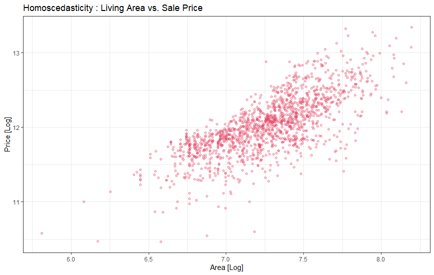

We plotted ‘SalePrice’ and ‘GrLivArea’ before but then why is the plot different? That’s right, because of the log transformation.

我們之前繪制了“ SalePrice”和“ GrLivArea”，但是為什么繪制不同？ 是的，因為有日志轉換。

If we go back to the previously plotted graphs showing the same variable, it is evident that the data has a conical shape when plotted. But after log transformation, the conic shape is no more. Here we solved the homoscedasticity problem with just one transformation. Pretty powerful eh?

如果我們回到顯示相同變量的先前繪制的圖，很明顯，繪制時數據具有圓錐形狀。 但是對數轉換后，圓錐形狀不再存在。 在這里，我們只用一種變換就解決了同方差問題。 很厲害嗎？

Now let’s check ‘SalePrice’ with ‘TotalBsmtSF’.

現在，讓我們用“ TotalBsmtSF”檢查“ SalePrice”。

ggplot(clean_data, aes(x=totalbsmt_log, y=log_price)) +
  theme_bw()+
  geom_point(colour="#e34262", alpha=0.3)+
  theme(legend.position='none')+
  labs(title = " Homoscedasticity : Total Basement Area vs. Sale Price", x="Area [Log]", y="Price [Log]")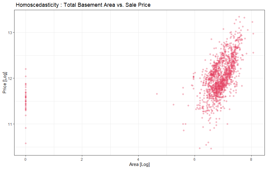

就是這樣，我們已經完成分析的結尾。 現在剩下的就是獲取虛擬變量了……其余的你都知道了。 :) (That’s it, we’ve reached the end of our Analysis. Now all that’s left is to get the dummy variables and… you know the rest. :))

This work was possible thanks to Pedro Marcelino. I found his Analysis on this dataset in Python and wanted to re-write it in R. Give him some love!

感謝Pedro Marcelino使得這項工作成為可能。 我在Python中找到了他對此數據集的分析，并想用R重新編寫它。給他一些愛！