By Aditya Pethe

通過阿蒂亞·皮特(Aditya Pethe)

From September to January every year, football takes over America. Games dominate TV Sunday and Monday nights, and my brother tears his hair out each week over his consistently underperforming fantasy teams. The hype seems to reach an unbearable level by the time the playoffs roll around.

每年的9月至1月，足球席卷美國。 游戲在星期日和星期一晚上占據著電視臺的主導地位，而我的兄弟每周都在表現不佳的幻想隊中大放異彩。 季后賽到來之時，炒作似乎已經到了難以忍受的地步。

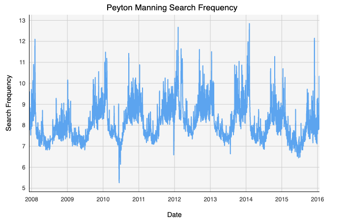
But is there a way to measure and forecast that hype? I decided to use one of my favorite NFL players, Peyton Manning, in order to explore seasonality in Deephaven’s Jupyter Notebooks. Using a dataset of Manning’s Wikipedia search frequencies taken over an 8 year period from 2008 to 2016, my goal was to break down how football hype evolved throughout the season.

但是，有沒有一種方法可以衡量和預測這種炒作？ 我決定使用我最喜歡的NFL球員之一Peyton Manning來探索Deephaven的Jupyter筆記本的季節性。 使用從2008年到2016年的8年期間內Manning的Wikipedia搜索頻率的數據集 ，我的目標是弄清整個賽季足球宣傳的演變。

To do this, I decided to take two approaches to analyzing seasonality. The first was the traditional ARIMA model, and the second was the newer Fbprophet library. I would use both these methods to fit, predict, and validate models to see which was better at understanding NFL hype.

為此，我決定采用兩種方法來分析季節性。 第一個是傳統的ARIMA模型，第二個是較新的Fbprophet庫。 我將使用這兩種方法來擬合，預測和驗證模型，以查看哪種方法更適合理解NFL宣傳。

我們的數據 (OUR DATA)

We can plot our data in Deephaven with the following code:

我們可以使用以下代碼在Deephaven中繪制數據：

At a top-level glance, our data is log-transformed Wikipedia page views for Peyton Manning taken each day for about 8 years. The data appears to exhibit some strong seasonal trends that we can look into.

從最高層次看，我們的數據是對Peyton Manning進行日志轉換的Wikipedia頁面視圖，大約每天進行8年。 數據似乎顯示出一些我們可以研究的強烈季節性趨勢。

Additionally, before we begin breaking down our data, we want a consistent way to visualize our forecasts. We can produce a function that takes our training, testing, and any forecast data and plots it with Deephaven. This allows us to combine analysis from multiple libraries and methods with Deephaven’s powerful and interactive plotting.

此外，在開始分解數據之前，我們需要一種一致的方式來可視化我們的預測。 我們可以產生一個函數，將我們的訓練，測試和所有預測數據都用Deephaven進行繪制。 這使我們能夠將來自多個庫和方法的分析與Deephaven強大而交互式的繪圖相結合。

有馬 (ARIMA)

The ARIMA model stands for autoregressive, integrated moving average model.

ARIMA模型代表自回歸，集成移動平均模型。

The Autoregressive, or AR component of the model, is a linear combination of the previous N seasonal lags. For our Peyton Manning model, this means some linear combination of the previous N weeks, months, or years.

模型的自回歸或AR分量是前N個季節滯后的線性組合。 對于我們的Peyton Manning模型，這意味著前N周，幾個月或幾年的線性組合。

The moving average component of the model is a linear combination of the error terms for the previous N seasonal lags, like so:

模型的移動平均成分是前N個季節滯后的誤差項的線性組合，如下所示：

The ARIMA model will estimate the coefficients for both these linear combinations, given three parameters as input:

給定三個參數作為輸入，ARIMA模型將估算這兩個線性組合的系數：

• p: The order of the autoregressive model (the number of lagged terms), described in the AR equation above.

  p：自回歸模型的順序(滯后項的數量)，在上面的AR方程中描述。

• q: The order of the moving average model (the number of lagged terms), described in the MA equation above.

  q：移動平均模型的階數(滯后項的數量)，如上面的MA方程所述。

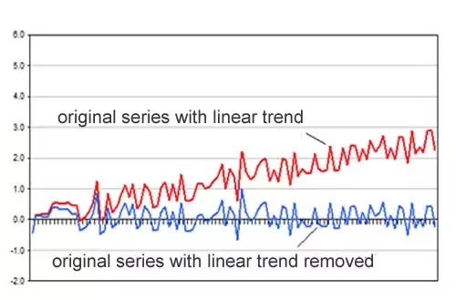
• d: The number of differences required to make the time series stationary. A stationary time series is essentially a time series without a time-dependent trend, excluding the seasonality.

  d：使時間序列固定所需的差數。 固定時間序列本質上是沒有季節性相關趨勢的時間序列，不包括季節性。

In the example below, the blue time series would be considered stationary, while the red would be nonstationary, even though both may exhibit seasonal patterns.

在下面的示例中，藍色時間序列將被認為是平穩的，而紅色時間序列將被視為非平穩的，即使這兩個時間序列都可能呈現季節性變化。

Now that we know what parameters we need to find, we can analyze our Peyton Manning data. At first glance, our data seems stationary. There doesn’t appear to be a time-dependent trend outside seasonal fluctuations, but we can test for this using the Augmented Dickey-Fuller Test.

既然我們知道需要找到什么參數，就可以分析Peyton Manning數據。 乍一看，我們的數據似乎穩定。 除季節性波動外，似乎沒有隨時間變化的趨勢，但是我們可以使用增強Dickey-Fuller檢驗進行檢驗。

Our test returns a p-value well below the significance level, so we can confirm that our model is indeed stationary. Our parameter value for d is zero.

我們的測試返回的p值遠低于顯著性水平，因此我們可以確認我們的模型確實是平穩的。 d的參數值為零。

Now we need to find the parameter values of P and Q. In order to do this, I used autocorrelation plots. Autocorrelation and partial autocorrelation plots can tell how strongly lagged terms correlated with a given observation. While partial autocorrelation plots tell the correlation with the lag term independent of other lags, autocorrelation plots factor in the “inertia” from other lags. Because of this, we can use partial autocorrelation to estimate our parameter for P, and autocorrelation to estimate our parameter for Q.

現在我們需要找到P和Q的參數值。為此，我使用了自相關圖。 自相關圖和局部自相關圖可以說明滯后項與給定觀察值的相關程度。 盡管部分自相關圖告訴了與滯后項的相關性，而與其他滯后無關，但自相關圖將其他滯后的“慣性”作為因素。 因此，我們可以使用偏自相關來估計P的參數，并使用自相關來估計Q的參數。

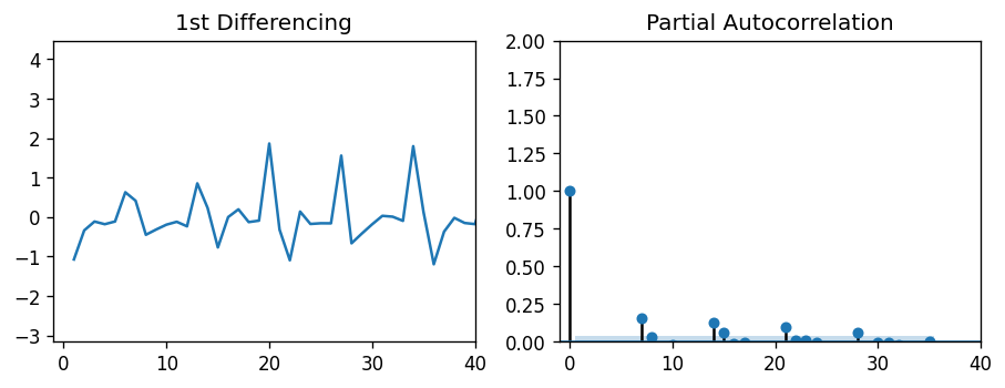
Both plots show a periodic behavior in the lags, each around 7 days in length. This makes sense — Peyton Manning search frequency probably increases on game nights, when football is being played. In fact, these autocorrelation plots even show a slight 6-day correlation, which is likely due to Sunday night football. But since the lags of 7 days have the highest correlation with the observed value, we can estimate both P and Q to be 7.

這兩個圖都顯示了滯后的周期性行為，每個周期的長度約為7天。 這是有道理的-在踢足球的比賽之夜，佩頓·曼寧的搜索頻率可能會增加。 實際上，這些自相關圖甚至顯示了輕微的6天相關性，這很可能是由于周日晚上的足球比賽所致。 但是由于7天的滯后與觀測值具有最高的相關性，因此我們可以估計P和Q均為7。

I should note that these autocorrelation plots presented a problem. The ARIMA parameters did not allow for lag inputs of over ~10, which meant that looking at annual (365) or monthly (30) seasonality would be very difficult.

我應該注意，這些自相關圖存在問題。 ARIMA參數不允許滯后輸入超過?10，這意味著查看年度(365)或每月(30)的季節性非常困難。

Now that we have our parameters, we can produce our ARIMA model.

現在我們有了參數，我們可以生成ARIMA模型。

Before we make our forecasts, we can check our model assumptions for variance and normality with a residual plot and density plot.

在進行預測之前，我們可以使用殘差圖和密度圖檢查模型假設的方差和正態性。

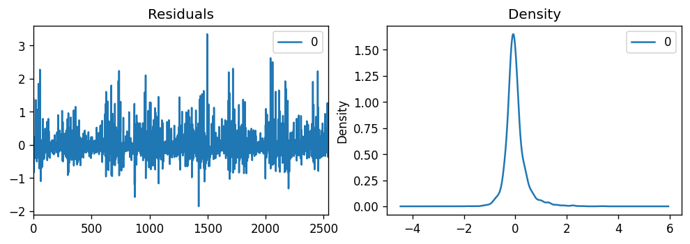
Since the residuals appear to be randomly distributed, and the kernel probability density plot appears normal, our model assumptions check out.

由于殘差似乎是隨機分布的，并且核概率密度圖似乎是正態的，因此我們的模型假設得到了檢驗。

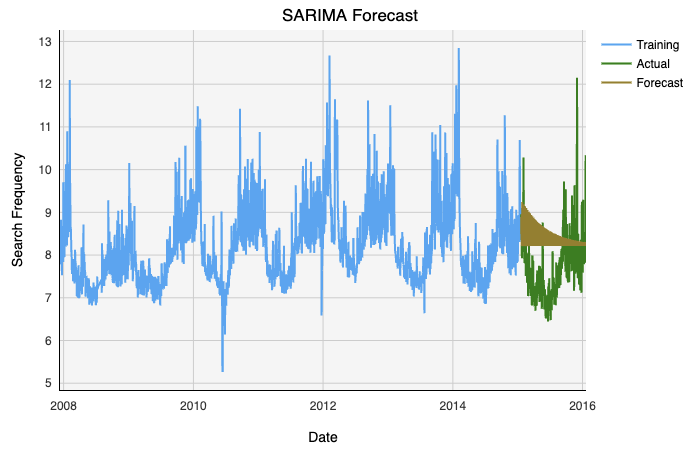
Plotting our model yields the following:

繪制模型將得出以下結果：

As we can see, not having access to the other scales of seasonality hurts this model’s viability. Not being able to capture multiple seasonal trends means that ARIMA is limited by one seasonality at a time. Regardless, we can return some error estimators to validate our model.

如我們所見，無法使用其他季節性尺度會損害該模型的生存能力。 無法捕獲多個季節趨勢意味著ARIMA一次只能受到一個季節的限制。 無論如何，我們可以返回一些誤差估計量來驗證我們的模型。

• MSE (mean squared error): 0.8916776825661407

  MSE (均方誤差)：0.8916776825661407

• MAPE (mean absolute percentage error): 0.10230290573107942

  MAPE (平均絕對百分比誤差)：0.10230290573107942

薩里瑪 (SARIMA)

We can actually validate our ARIMA model using the auto-SARIMA model from pmdarima. The auto-SARIMA model estimates the parameter values for p, q, and d for us so there is no need for the prelude above. In addition, SARIMA takes m, the period of seasonality, as a parameter. Unfortunately, the model parameter limitations again constrain us to m < 10, so we may only look at weekly seasonality.

實際上，我們可以使用pmdarima的auto-SARIMA模型驗證ARIMA模型。 auto-SARIMA模型為我們估計p ， q和d的參數值，因此不需要上面的前奏。 另外，SARIMA將季節周期m用作參數。 不幸的是，模型參數限制再次將我們限制為m <10 ，因此我們可能只查看每周的季節性。

Fitting and plotting our model gives us the following:

擬合和繪制模型可以得到以下結果：

Lastly, we can validate our model with error metrics:

最后，我們可以使用錯誤指標來驗證我們的模型：

• MSE (mean squared error): 0.8916776825661407

  MSE (均方誤差)：0.8916776825661407

• MAPE (mean absolute percentage error): 0.10789283997956421

  MAPE (平均絕對百分比誤差)：0.10789283997956421

We see that our SARIMA model performed nearly identically to our ARIMA model, and in fact our ARIMA model gave a slightly lower mean absolute percentage error than SARIMA. We can be happy that we picked optimal parameters to fit our ARIMA model with.

我們看到，SARIMA模型的性能幾乎與ARIMA模型相同，并且實際上，ARIMA模型的平均絕對百分比誤差略低于SARIMA。 我們很高興選擇了適合ARIMA模型的最佳參數。

預言家 (PROPHET)

For our final model, we will be using Fbprophet.

對于我們的最終模型，我們將使用Fbprophet。

Fbprophet is a library from Facebook intended to handle seasonal time-series datasets. Prophet implements a procedure for forecasting time series data based on an additive model where non-linear trends are fit with yearly, weekly, and daily seasonality, plus holiday effects. In general, using Prophet requires much less hands-on work than our ARIMA model, and for the most part, we can feed our data directly into prophet like so:

Fbprophet是Facebook的一個庫，用于處理季節性時間序列數據集。 先知實現了一種基于加性模型的時間序列數據預測程序，其中非線性趨勢與年，周和日的季節性以及假期效應相吻合。 通常，與我們的ARIMA模型相比，使用Prophet所需的動手工作少得多，并且在大多數情況下，我們可以像這樣將數據直接輸入到先知中：

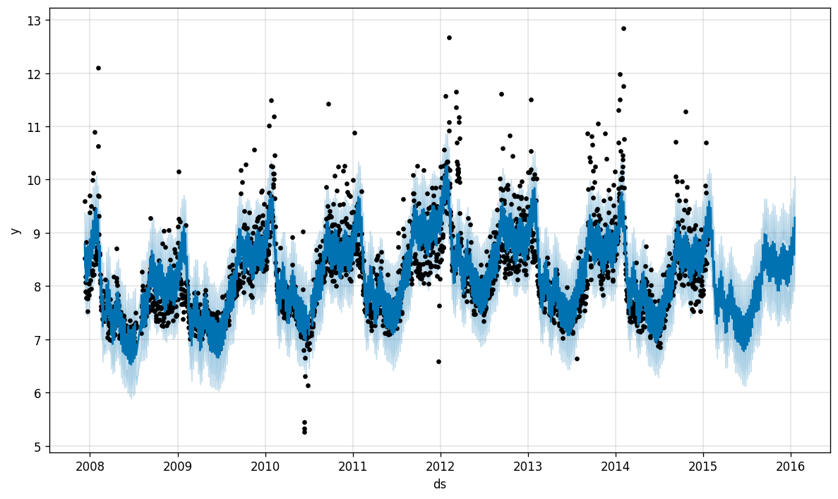
This allows us to forecast one year ahead, and compare actual data with expected values and their boundaries.

這使我們可以預測一年，并將實際數據與期望值及其界限進行比較。

In addition, Prophet allows us to break down this data into seasonal components:

此外，先知使我們可以將這些數據分解為季節性成分：

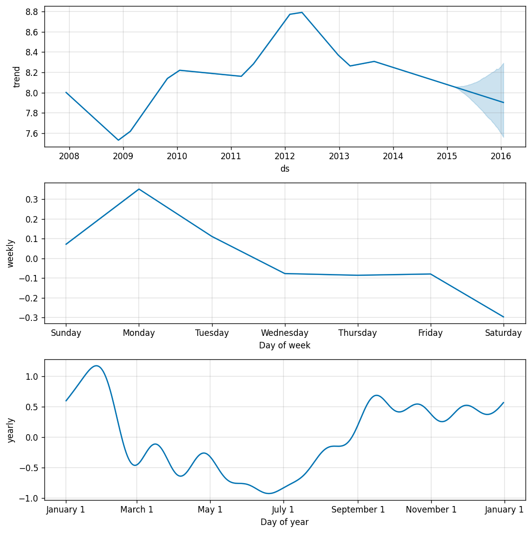
Manning’s page views peaked in 2012–2013, his MVP year. Unsurprisingly, Monday night football is when most fans look Manning up, and the monthly seasonal breakdown shows the crazy highs of December and March in stark contrast to the great drought of the summer.

曼寧的網頁瀏覽量在他的MVP年度(2012-2013)達到頂峰。 毫不奇怪，周一晚上的足球比賽是大多數球迷抬頭看曼寧的時候，每月的季節性故障顯示出12月和3月的瘋狂高點，與夏季的干旱形成鮮明對比。

Prophet can do even more, and add changepoints to the data, where the trend is most likely to shift.

先知可以做更多的事情，并且可以向數據添加變化點，而趨勢最有可能在此變化。

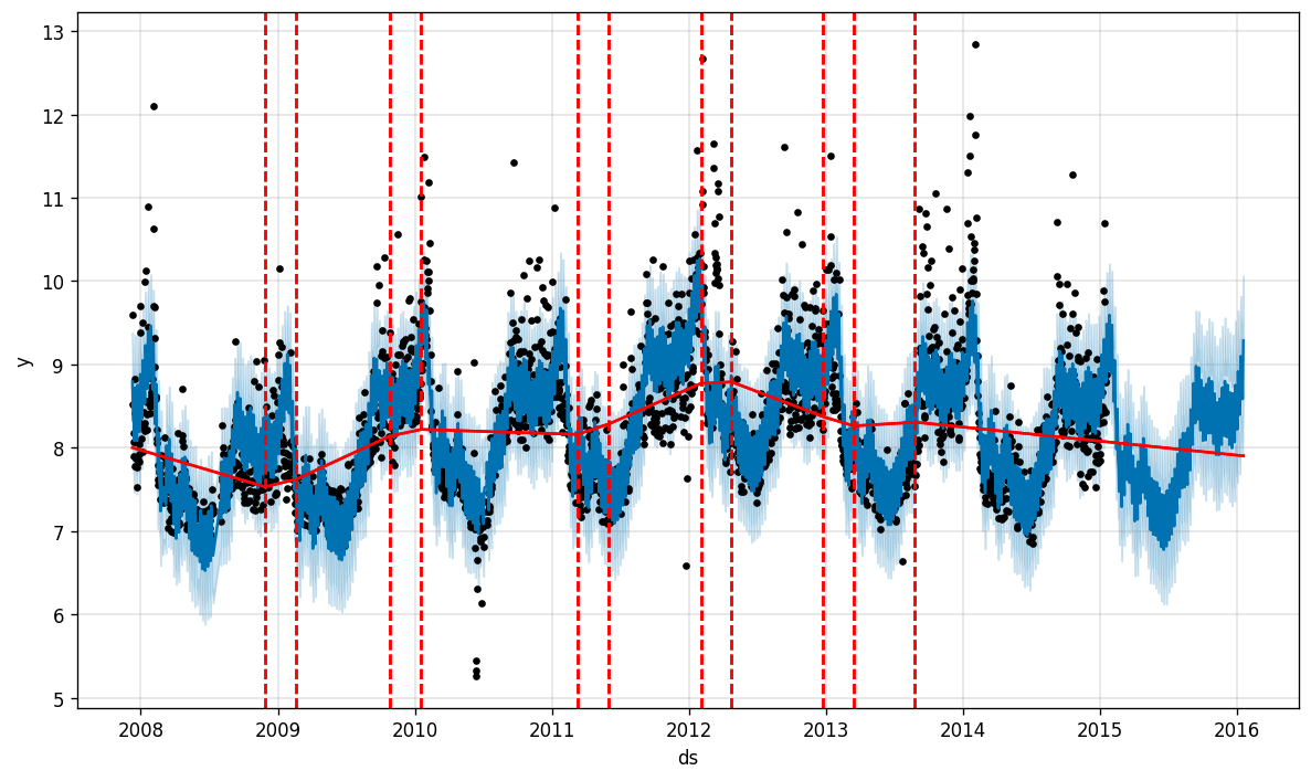
With this feature, Prophet roughly estimates the start and end of the season, especially capturing the window of the playoffs.

通過此功能，先知大致估計了賽季的開始和結束，尤其是捕獲了季后賽的窗口。

By the eye test alone, our prophet models look much better and coherent than ARIMA. But we can again validate the model predictions using MSE and MAPE.

僅憑眼睛測試，我們的先知模型看上去比ARIMA更好，更連貫。 但是我們可以再次使用MSE和MAPE驗證模型預測。

• MSE (mean squared error): 0.35800021765342394

  MSE (均方誤差)：0.35800021765342394

• MAPE (mean absolute percentage error): 0.059460265364126956

  MAPE (平均絕對百分比誤差)：0.059460265364126956

結論 (CONCLUSION)

Both error estimators clearly point to Prophet as the more accurate model. For large time-series data with multiple seasonalities, ARIMA has many shortcomings. Simply using regression on previous lags to estimate future values won’t cut it in predicting more complex time-series datasets. ARIMA may be useful for more limited datasets with simpler seasonal effects, but particularly for things like sensor data, page views, or energy consumption, complex nonlinear models like Prophet are required to make predictions.

兩種誤差估計器都明確指出先知是更準確的模型。 對于具有多個季節性的大型時間序列數據，ARIMA有許多缺點。 只需對先前的滯后使用回歸來估計未來值，就無法預測更復雜的時間序列數據集。 ARIMA可能對于季節效應較為簡單的有限數據集很有用，但是對于傳感器數據，頁面瀏覽量或能源消耗之類的東西尤其如此，需要使用諸如Prophet之類的復雜非線性模型進行預測。

Deephaven’s integration with Jupyter Notebooks allows for users to have unique, library-specific plotting methods and operations side by side with Deephaven features. Deephaven’s plotting in particular provides user-friendly visualization options in interactive plots when used in conjunction with new, cutting edge libraries like fbprophet.

Deephaven與Jupyter Notebooks的集成使用戶可以與Deephaven功能并排使用獨特的，特定于庫的繪圖方法和操作。 當與新的尖端庫(例如fbprophet)結合使用時，Deephaven的繪圖在交互式繪圖中尤其提供了用戶友好的可視化選項。