所有代碼塊都是在Jupyter Notebook下進行調試運行，前后之間都相互關聯。
文中所有代碼塊所涉及到的函數里面的詳細參數均可通過scikit-learn官網API文檔進行查閱，這里我只寫下每行代碼所實現的功能，參數的調整讀者可以多進行試驗調試。多動手！！！

一、簡介

線性回歸是回歸問題，可以得到一個具體的回歸值；而邏輯回歸是分類問題，可以得到將兩種類別物體分類。
邏輯回歸借助sigmoid函數進行了數值映射，將求出的值轉換為0-1之間的概率，通過比較相關概率從而實現分類任務。

導包

import numpy as np
import os
%matplotlib inline
import matplotlib
import matplotlib.pyplot as plt
plt.rcParams['axes.labelsize'] = 14
plt.rcParams['xtick.labelsize'] = 12
plt.rcParams['ytick.labelsize'] = 12
import warnings
warnings.filterwarnings('ignore')
np.random.seed(42)

二、sigmoid函數

t = np.linspace(-10, 10, 100)
sig = 1 / (1 + np.exp(-t))
plt.figure(figsize=(9, 3))
plt.plot([-10, 10], [0, 0], "k-")
plt.plot([-10, 10], [0.5, 0.5], "k:")
plt.plot([-10, 10], [1, 1], "k:")
plt.plot([0, 0], [-1.1, 1.1], "k-")
plt.plot(t, sig, "b-", linewidth=2, label=r"$\sigma(t) = \frac{1}{1 + e^{-t}}$")
plt.xlabel("t")
plt.legend(loc="upper left", fontsize=20)
plt.axis([-10, 10, -0.1, 1.1])
plt.title('Figure 4-21. Logistic function')
plt.show()

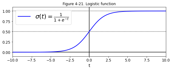
其對應的相關推導公式如下：

三、鳶尾花數據集

這個鳶尾花數據集是sklearn庫里面自帶的數據集，主要由三個類別的花，每種類別的花都有四個特征參數。
邏輯回歸可以實現二分類問題，對于三分類問題，只需要將剩余其他兩種類別的花當成一種(當成其他即可)，依次分別進行三次二分類就可以實現三分類的任務。

Ⅰ，加載iris(鳶尾花)數據集

from sklearn import datasets
iris = datasets.load_iris()
list(iris.keys())#查看數據集中都有哪些屬性可以調用，這里主要使用data---x，target---y
"""
['data','target','frame','target_names','DESCR','feature_names','filename']
"""

Ⅱ，查看iris數據集的詳細信息描述

print (iris.DESCR)#當前iris鳶尾花數據集的所有信息的描述
"""
.. _iris_dataset:Iris plants dataset
--------------------**Data Set Characteristics:**:Number of Instances: 150 (50 in each of three classes):Number of Attributes: 4 numeric, predictive attributes and the class:Attribute Information:- sepal length in cm- sepal width in cm- petal length in cm- petal width in cm- class:- Iris-Setosa- Iris-Versicolour- Iris-Virginica:Summary Statistics:============== ==== ==== ======= ===== ====================Min  Max   Mean    SD   Class Correlation============== ==== ==== ======= ===== ====================sepal length:   4.3  7.9   5.84   0.83    0.7826sepal width:    2.0  4.4   3.05   0.43   -0.4194petal length:   1.0  6.9   3.76   1.76    0.9490  (high!)petal width:    0.1  2.5   1.20   0.76    0.9565  (high!)============== ==== ==== ======= ===== ====================:Missing Attribute Values: None:Class Distribution: 33.3% for each of 3 classes.:Creator: R.A. Fisher:Donor: Michael Marshall (MARSHALL%PLU@io.arc.nasa.gov):Date: July, 1988The famous Iris database, first used by Sir R.A. Fisher. The dataset is taken
from Fisher's paper. Note that it's the same as in R, but not as in the UCI
Machine Learning Repository, which has two wrong data points.This is perhaps the best known database to be found in the
pattern recognition literature.  Fisher's paper is a classic in the field and
is referenced frequently to this day.  (See Duda & Hart, for example.)  The
data set contains 3 classes of 50 instances each, where each class refers to a
type of iris plant.  One class is linearly separable from the other 2; the
latter are NOT linearly separable from each other... topic:: References- Fisher, R.A. "The use of multiple measurements in taxonomic problems"Annual Eugenics, 7, Part II, 179-188 (1936); also in "Contributions toMathematical Statistics" (John Wiley, NY, 1950).- Duda, R.O., & Hart, P.E. (1973) Pattern Classification and Scene Analysis.(Q327.D83) John Wiley & Sons.  ISBN 0-471-22361-1.  See page 218.- Dasarathy, B.V. (1980) "Nosing Around the Neighborhood: A New SystemStructure and Classification Rule for Recognition in Partially ExposedEnvironments".  IEEE Transactions on Pattern Analysis and MachineIntelligence, Vol. PAMI-2, No. 1, 67-71.- Gates, G.W. (1972) "The Reduced Nearest Neighbor Rule".  IEEE Transactionson Information Theory, May 1972, 431-433.- See also: 1988 MLC Proceedings, 54-64.  Cheeseman et al"s AUTOCLASS IIconceptual clustering system finds 3 classes in the data.- Many, many more ..."""

Ⅲ，選出其中一種類別的花，將其余兩種花分為一類

X = iris['data'][:,3:]#選出所有數據中的其中一個特征
y = (iris['target'] == 2).astype(np.int)#將這種花設定為1，剩下的兩種花設定為0

y#很顯然，前面的0為其余兩種花，后面的1是當前這種花
"""
array([0, 0, 0, 0, 0, 0, 0, 0, 0, 0, 0, 0, 0, 0, 0, 0, 0, 0, 0, 0, 0, 0,0, 0, 0, 0, 0, 0, 0, 0, 0, 0, 0, 0, 0, 0, 0, 0, 0, 0, 0, 0, 0, 0,0, 0, 0, 0, 0, 0, 0, 0, 0, 0, 0, 0, 0, 0, 0, 0, 0, 0, 0, 0, 0, 0,0, 0, 0, 0, 0, 0, 0, 0, 0, 0, 0, 0, 0, 0, 0, 0, 0, 0, 0, 0, 0, 0,0, 0, 0, 0, 0, 0, 0, 0, 0, 0, 0, 0, 1, 1, 1, 1, 1, 1, 1, 1, 1, 1,1, 1, 1, 1, 1, 1, 1, 1, 1, 1, 1, 1, 1, 1, 1, 1, 1, 1, 1, 1, 1, 1,1, 1, 1, 1, 1, 1, 1, 1, 1, 1, 1, 1, 1, 1, 1, 1, 1, 1])
"""

Ⅳ，訓練模型及展示

①模型訓練

from sklearn.linear_model import LogisticRegression#導入邏輯回歸包
log_res = LogisticRegression()#實例化
log_res.fit(X,y)#傳入參數訓練模型
"""
LogisticRegression(C=1.0, class_weight=None, dual=False, fit_intercept=True,intercept_scaling=1, max_iter=100, multi_class='warn',n_jobs=None, penalty='l2', random_state=None, solver='warn',tol=0.0001, verbose=0, warm_start=False)
"""

X_new = np.linspace(0,3,1000).reshape(-1,1)#從0-3取1000個數
y_proba = log_res.predict_proba(X_new)#得出預測結果

y_proba#得出1000個樣本通過模型得出的概率值，左邊表示屬于當前類別的概率，右邊表示不屬于當前類別的概率
"""
array([[0.98554411, 0.01445589],[0.98543168, 0.01456832],[0.98531838, 0.01468162],...,[0.02618938, 0.97381062],[0.02598963, 0.97401037],[0.02579136, 0.97420864]])
"""

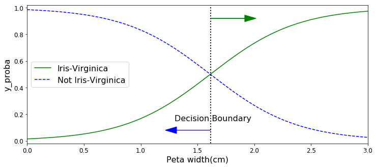
②可視化展示

plt.figure(figsize=(12,5))#整個一張圖繪制
decision_boundary = X_new[y_proba[:,1]>=0.5][0]#指定決策邊界所處的位置
plt.plot([decision_boundary,decision_boundary],[-1,2],'k:',linewidth = 2)#將邊界從上往下繪制
plt.plot(X_new,y_proba[:,1],'g-',label = 'Iris-Virginica')#是當前類別的花
plt.plot(X_new,y_proba[:,0],'b--',label = 'Not Iris-Virginica')#不是當前類別的花
plt.arrow(decision_boundary,0.08,-0.3,0,head_width = 0.05,head_length=0.1,fc='b',ec='b')#指定箭頭
plt.arrow(decision_boundary,0.92,0.3,0,head_width = 0.05,head_length=0.1,fc='g',ec='g')
plt.text(decision_boundary+0.02,0.15,'Decision Boundary',fontsize = 16,color = 'k',ha='center')#添加字符串指定決策邊界
plt.xlabel('Peta width(cm)',fontsize = 16)#x軸標簽，花瓣寬度
plt.ylabel('y_proba',fontsize = 16)#y軸標簽，最終預測的概率值
plt.axis([0,3,-0.02,1.02])#設置x和y軸的取值范圍
plt.legend(loc = 'center left',fontsize = 16)#顯示標簽，放在中間偏左位置

遇到不太熟悉的函數，比如畫箭頭arrow，可以通過查閱幫助文檔進行解決

print (help(plt.arrow))
"""
Help on function arrow in module matplotlib.pyplot:arrow(x, y, dx, dy, **kwargs)Add an arrow to the axes.This draws an arrow from ``(x, y)`` to ``(x+dx, y+dy)``.Parameters----------x, y : floatThe x/y-coordinate of the arrow base.dx, dy : floatThe length of the arrow along x/y-direction.Returns-------arrow : `.FancyArrow`The created `.FancyArrow` object.Other Parameters----------------**kwargsOptional kwargs (inherited from `.FancyArrow` patch) control thearrow construction and properties:Constructor arguments*width*: float (default: 0.001)width of full arrow tail*length_includes_head*: bool (default: False)True if head is to be counted in calculating the length.*head_width*: float or None (default: 3*width)total width of the full arrow head*head_length*: float or None (default: 1.5 * head_width)length of arrow head*shape*: ['full', 'left', 'right'] (default: 'full')draw the left-half, right-half, or full arrow*overhang*: float (default: 0)fraction that the arrow is swept back (0 overhang meanstriangular shape). Can be negative or greater than one.*head_starts_at_zero*: bool (default: False)if True, the head starts being drawn at coordinate 0instead of ending at coordinate 0.Other valid kwargs (inherited from :class:`Patch`) are:agg_filter: a filter function, which takes a (m, n, 3) float array and a dpi value, and returns a (m, n, 3) array alpha: float or Noneanimated: boolantialiased: unknowncapstyle: {'butt', 'round', 'projecting'}clip_box: `.Bbox`clip_on: boolclip_path: [(`~matplotlib.path.Path`, `.Transform`) | `.Patch` | None] color: colorcontains: callableedgecolor: color or None or 'auto'facecolor: color or Nonefigure: `.Figure`fill: boolgid: strhatch: {'/', '\\', '|', '-', '+', 'x', 'o', 'O', '.', '*'}in_layout: booljoinstyle: {'miter', 'round', 'bevel'}label: objectlinestyle: {'-', '--', '-.', ':', '', (offset, on-off-seq), ...}linewidth: float or None for default path_effects: `.AbstractPathEffect`picker: None or bool or float or callablerasterized: bool or Nonesketch_params: (scale: float, length: float, randomness: float) snap: bool or Nonetransform: `.Transform`url: strvisible: boolzorder: floatNotes-----The resulting arrow is affected by the axes aspect ratio and limits.This may produce an arrow whose head is not square with its stem. Tocreate an arrow whose head is square with its stem,use :meth:`annotate` for example:>>> ax.annotate("", xy=(0.5, 0.5), xytext=(0, 0),...             arrowprops=dict(arrowstyle="->"))None
"""

Ⅴ，笛卡爾積(棋盤操作)樣例

x0,x1 = np.meshgrid(np.linspace(1,2,2).reshape(-1,1),np.linspace(10,20,3).reshape(-1,1))#笛卡爾積

x0
"""
array([[1., 2.],[1., 2.],[1., 2.]])
"""

x1
"""
array([[10., 10.],[15., 15.],[20., 20.]])
"""

np.c_[x0.ravel(),x1.ravel()]#拼接
"""
array([[ 1., 10.],[ 2., 10.],[ 1., 15.],[ 2., 15.],[ 1., 20.],[ 2., 20.]])
"""

從運行結果也不難看出，笛卡爾積的操作就類似一個棋盤，(1，2，2)也就是從1-2之間選取2個數賦值給x0，(10，20，3)從10到20之間選取3個數賦值給x1。
拼接之后即可得到這幾個數的全部的排列組合情況。

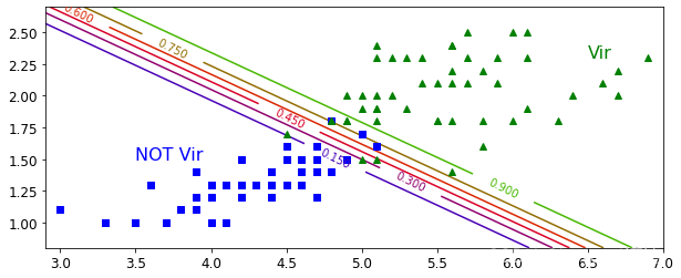
Ⅵ，分類決策邊界

X[:,0].min(),X[:,0].max()#獲取標簽為0的數據的大致范圍為后續的畫圖做參考
"""
(1.0, 6.9)
"""

X[:,1].min(),X[:,1].max()#獲取標簽為1的數據的大致范圍為后續的畫圖做參考
"""
(0.1, 2.5)
"""

x0,x1 = np.meshgrid(np.linspace(2.9,7,500).reshape(-1,1),np.linspace(0.8,2.7,200).reshape(-1,1))

X_new = np.c_[x0.ravel(),x1.ravel()]#拼接
X_new#獲得測試數據
"""
array([[2.9       , 0.8       ],[2.90821643, 0.8       ],[2.91643287, 0.8       ],...,[6.98356713, 2.7       ],[6.99178357, 2.7       ],[7.        , 2.7       ]])
"""

X_new.shape#100000=500*200
"""
(100000, 2)
"""

y_proba = log_res.predict_proba(X_new)#通過訓練好的模型去預測測試數據的概率值

x0.shape#維度參數得與后續z軸一致
"""
(200, 500)
"""

x1.shape#維度參數得與后續z軸一致
"""
(200, 500)
"""

plt.figure(figsize=(10,4))#繪制圖片的框架大小
plt.plot(X[y==0,0],X[y==0,1],'bs')#展示數據點
plt.plot(X[y==1,0],X[y==1,1],'g^')#展示數據點zz = y_proba[:,1].reshape(x0.shape)#繪制z軸
contour = plt.contour(x0,x1,zz,cmap=plt.cm.brg)#繪制等高線
plt.clabel(contour,inline = 1)#等高線上添加概率值
plt.axis([2.9,7,0.8,2.7])#限制x和y軸的取值范圍
plt.text(3.5,1.5,'NOT Vir',fontsize = 16,color = 'b')#展示標簽
plt.text(6.5,2.3,'Vir',fontsize = 16,color = 'g')#展示標簽

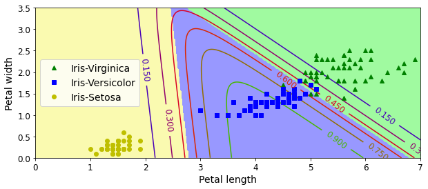
四、Softmax

如何實現之間對多列別進行分類，這里Softmax就派上用場了。

由公式很明顯可知，softmax實際上就是先對數據求指數，然后目的就是為了拉大差距，之后再進行歸一化操作。
損失函數也就是對數，0-1之間聯想下對數函數。

X = iris['data'][:,(2,3)]#獲取數據
y = iris['target']#獲取標簽

softmax_reg = LogisticRegression(multi_class = 'multinomial',solver='lbfgs')#指定多分類，指定求解的方法
softmax_reg.fit(X,y)#訓練
"""
LogisticRegression(C=1.0, class_weight=None, dual=False, fit_intercept=True,intercept_scaling=1, max_iter=100, multi_class='multinomial',n_jobs=None, penalty='l2', random_state=None, solver='lbfgs',tol=0.0001, verbose=0, warm_start=False)
"""

softmax_reg.predict([[5,2]])#二維數據
"""
array([2])
"""

softmax_reg.predict_proba([[5,2]])#預測看看有幾個概率值，也就是分成了幾類，也就證實了這是個多分類的任務
"""
array([[2.43559894e-04, 2.14859516e-01, 7.84896924e-01]])
"""

#繪制等高線
x0, x1 = np.meshgrid(np.linspace(0, 8, 500).reshape(-1, 1),np.linspace(0, 3.5, 200).reshape(-1, 1),)
X_new = np.c_[x0.ravel(), x1.ravel()]y_proba = softmax_reg.predict_proba(X_new)
y_predict = softmax_reg.predict(X_new)zz1 = y_proba[:, 1].reshape(x0.shape)
zz = y_predict.reshape(x0.shape)plt.figure(figsize=(10, 4))
plt.plot(X[y==2, 0], X[y==2, 1], "g^", label="Iris-Virginica")
plt.plot(X[y==1, 0], X[y==1, 1], "bs", label="Iris-Versicolor")
plt.plot(X[y==0, 0], X[y==0, 1], "yo", label="Iris-Setosa")from matplotlib.colors import ListedColormap
custom_cmap = ListedColormap(['#fafab0','#9898ff','#a0faa0'])plt.contourf(x0, x1, zz, cmap=custom_cmap)
contour = plt.contour(x0, x1, zz1, cmap=plt.cm.brg)
plt.clabel(contour, inline=1, fontsize=12)
plt.xlabel("Petal length", fontsize=14)
plt.ylabel("Petal width", fontsize=14)
plt.legend(loc="center left", fontsize=14)
plt.axis([0, 7, 0, 3.5])
plt.show()