我看過很多課程，不過內容都大差不差，也可以參考這篇模型評估方法

一、K折交叉驗證

一般情況，我們得到一份數據集，會分為兩類，一類是trainset訓練集，另一類十testset測試集。通俗一點也就是訓練集相當于平常的練習冊，直接去刷題；測試集就是高考，只有一次！而且還沒見過。但是一味的刷題真的好嗎？

這時，交叉驗證(Cross-validation)出現了，也成為CV，啥意思呢？就是將訓練集再進行劃分為trainset訓練集和validset驗證集，驗證集去充當期末考試，這是不是就合理多了。
例如：1000份數據，原本是200測試集、800訓練集；當交叉驗證引進之后就變成了200測試集、600訓練集、200驗證集。這里的驗證集是從原本的訓練集中來的。
800訓練集，通過交叉驗證分為了600訓練集、200驗證集，也就是分成了四份，這就是四折交叉驗證。同理將訓練集分成幾份就是幾折交叉驗證。一般情況驗證集占一份即可。

交叉驗證(Cross-validation)主要應用于建模中，例如PCR、PLS回歸建模，在給定的建模樣本中，留出一小部分，用剛訓練出來的模型進行預測，并求出這小部分的樣本預測誤差，記錄一下平方加和。

實時上，模型中有很多的超參數需要用戶進行傳入，不單單是學習率α一個，還有收斂閾值、泛化能力值等，這時候咋辦捏？GridSearchCV來了！

二、GridSearchCV

這玩意兒其實就是個函數，很厲害啊，別小看人家。它可以將你傳入的多個超參數進行排列組合，然后代入模型中進行訓練，最后返回出效果最佳的超參數。這就不需要人為的去傻了吧唧的一個一個的調參選出最優解了。
GridSearchCV(log_reg, param_grid=param_grid, cv=3)
第一個參數：要對哪一個模型進行訓練
第二個參數：選擇的超參數有哪些
第三個參數：幾折交叉驗證

三、代碼實戰

import numpy as np
from sklearn import datasets
from sklearn.linear_model import LogisticRegression
from sklearn.model_selection import GridSearchCV
import matplotlib.pyplot as plt
from time import timeiris = datasets.load_iris()
#print(list(iris.keys()))
#print(iris['DESCR'])
#print(iris['feature_names'])#特征名X = iris['data'][:, 3:]#取出x矩陣
#print(X)#petal width(cm)#print(iris['target'])
y = iris['target']
# y = (iris['target'] == 2).astype(np.int)
#print(y)#獲取類別號# Utility function to report best scores
def report(results, n_top=3):for i in range(1, n_top + 1):candidates = np.flatnonzero(results['rank_test_score'] == i)for candidate in candidates:print("Model with rank: {0}".format(i))print("Mean validation score: {0:.3f} (std: {1:.3f})".format(results['mean_test_score'][candidate],results['std_test_score'][candidate]))print("Parameters: {0}".format(results['params'][candidate]))print("")start = time()
# tol收斂的閾值超參數
# C泛化能力，越小泛化能力越高
param_grid = {"tol": [1e-4, 1e-3, 1e-2],"C": [0.4, 0.6, 0.8]}
log_reg = LogisticRegression(multi_class='ovr', solver='sag')#多個二分類來解決多分類為ovr，若為multinomial則使用softmax求解多分類問題；梯度下降法sag；
grid_search = GridSearchCV(log_reg, param_grid=param_grid, cv=3)
"""
GridSearchCV函數
第一個參數：要對哪一個模型進行訓練
第二個參數：選擇的超參數有哪些
第三個參數：幾折交叉驗證
"""
grid_search.fit(X, y)
print("GridSearchCV took %.2f seconds for %d candidate parameter settings."% (time() - start, len(grid_search.cv_results_['params'])))
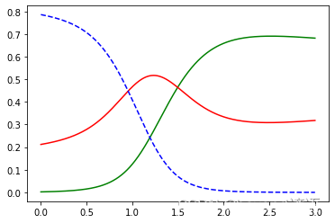
report(grid_search.cv_results_)X_new = np.linspace(0, 3, 1000).reshape(-1, 1)#創建新的數據集，從0-3這個區間范圍內，取1000個數值，linspace為平均分成1000個段，取出1000個點
#print(X_new)y_proba = grid_search.predict_proba(X_new)#預測分類號具體分類成哪一個類別的概率值
y_hat = grid_search.predict(X_new)#預測分類號具體分類成哪一個類別，跟0.5去比較，從而劃分為0或者1
print(y_proba)
print(y_hat)
print("w1",grid_search.best_estimator_)plt.plot(X_new, y_proba[:, 2], 'g-', label='Iris-Virginica')
plt.plot(X_new, y_proba[:, 1], 'r-', label='Iris-Versicolour')
plt.plot(X_new, y_proba[:, 0], 'b--', label='Iris-Setosa')
plt.show()print(grid_search.predict([[1.7], [1.5]]))
"""
GridSearchCV took 0.05 seconds for 9 candidate parameter settings.
Model with rank: 1
Mean validation score: 0.907 (std: 0.025)
Parameters: {'C': 0.6, 'tol': 0.0001}Model with rank: 1
Mean validation score: 0.907 (std: 0.025)
Parameters: {'C': 0.6, 'tol': 0.001}Model with rank: 1
Mean validation score: 0.907 (std: 0.025)
Parameters: {'C': 0.6, 'tol': 0.01}Model with rank: 1
Mean validation score: 0.907 (std: 0.025)
Parameters: {'C': 0.8, 'tol': 0.0001}Model with rank: 1
Mean validation score: 0.907 (std: 0.025)
Parameters: {'C': 0.8, 'tol': 0.001}Model with rank: 1
Mean validation score: 0.907 (std: 0.025)
Parameters: {'C': 0.8, 'tol': 0.01}[[7.85881224e-01 2.11932164e-01 2.18661232e-03][7.85645909e-01 2.12143369e-01 2.21072210e-03][7.85409133e-01 2.12355759e-01 2.23510765e-03]...[1.25568737e-04 3.17858272e-01 6.82016160e-01][1.24101822e-04 3.17945561e-01 6.81930337e-01][1.22652125e-04 3.18033028e-01 6.81844320e-01]]
[0 0 0 0 0 0 0 0 0 0 0 0 0 0 0 0 0 0 0 0 0 0 0 0 0 0 0 0 0 0 0 0 0 0 0 0 00 0 0 0 0 0 0 0 0 0 0 0 0 0 0 0 0 0 0 0 0 0 0 0 0 0 0 0 0 0 0 0 0 0 0 0 00 0 0 0 0 0 0 0 0 0 0 0 0 0 0 0 0 0 0 0 0 0 0 0 0 0 0 0 0 0 0 0 0 0 0 0 00 0 0 0 0 0 0 0 0 0 0 0 0 0 0 0 0 0 0 0 0 0 0 0 0 0 0 0 0 0 0 0 0 0 0 0 00 0 0 0 0 0 0 0 0 0 0 0 0 0 0 0 0 0 0 0 0 0 0 0 0 0 0 0 0 0 0 0 0 0 0 0 00 0 0 0 0 0 0 0 0 0 0 0 0 0 0 0 0 0 0 0 0 0 0 0 0 0 0 0 0 0 0 0 0 0 0 0 00 0 0 0 0 0 0 0 0 0 0 0 0 0 0 0 0 0 0 0 0 0 0 0 0 0 0 0 0 0 0 0 0 0 0 0 00 0 0 0 0 0 0 0 0 0 0 0 0 0 0 0 0 0 0 0 0 0 0 0 0 0 0 0 0 0 0 0 0 0 0 0 00 0 0 0 0 0 0 0 0 0 0 0 0 0 0 0 0 0 0 0 0 0 1 1 1 1 1 1 1 1 1 1 1 1 1 1 11 1 1 1 1 1 1 1 1 1 1 1 1 1 1 1 1 1 1 1 1 1 1 1 1 1 1 1 1 1 1 1 1 1 1 1 11 1 1 1 1 1 1 1 1 1 1 1 1 1 1 1 1 1 1 1 1 1 1 1 1 1 1 1 1 1 1 1 1 1 1 1 11 1 1 1 1 1 1 1 1 1 1 1 1 1 1 1 1 1 1 1 1 1 1 1 1 1 1 1 1 1 1 1 1 1 1 1 11 1 1 1 1 1 1 1 1 1 1 1 1 1 1 1 1 1 1 1 1 1 1 1 1 1 1 1 1 1 1 1 1 1 1 1 11 1 1 1 1 1 1 1 1 1 1 1 1 1 1 1 1 1 2 2 2 2 2 2 2 2 2 2 2 2 2 2 2 2 2 2 22 2 2 2 2 2 2 2 2 2 2 2 2 2 2 2 2 2 2 2 2 2 2 2 2 2 2 2 2 2 2 2 2 2 2 2 22 2 2 2 2 2 2 2 2 2 2 2 2 2 2 2 2 2 2 2 2 2 2 2 2 2 2 2 2 2 2 2 2 2 2 2 22 2 2 2 2 2 2 2 2 2 2 2 2 2 2 2 2 2 2 2 2 2 2 2 2 2 2 2 2 2 2 2 2 2 2 2 22 2 2 2 2 2 2 2 2 2 2 2 2 2 2 2 2 2 2 2 2 2 2 2 2 2 2 2 2 2 2 2 2 2 2 2 22 2 2 2 2 2 2 2 2 2 2 2 2 2 2 2 2 2 2 2 2 2 2 2 2 2 2 2 2 2 2 2 2 2 2 2 22 2 2 2 2 2 2 2 2 2 2 2 2 2 2 2 2 2 2 2 2 2 2 2 2 2 2 2 2 2 2 2 2 2 2 2 22 2 2 2 2 2 2 2 2 2 2 2 2 2 2 2 2 2 2 2 2 2 2 2 2 2 2 2 2 2 2 2 2 2 2 2 22 2 2 2 2 2 2 2 2 2 2 2 2 2 2 2 2 2 2 2 2 2 2 2 2 2 2 2 2 2 2 2 2 2 2 2 22 2 2 2 2 2 2 2 2 2 2 2 2 2 2 2 2 2 2 2 2 2 2 2 2 2 2 2 2 2 2 2 2 2 2 2 22 2 2 2 2 2 2 2 2 2 2 2 2 2 2 2 2 2 2 2 2 2 2 2 2 2 2 2 2 2 2 2 2 2 2 2 22 2 2 2 2 2 2 2 2 2 2 2 2 2 2 2 2 2 2 2 2 2 2 2 2 2 2 2 2 2 2 2 2 2 2 2 22 2 2 2 2 2 2 2 2 2 2 2 2 2 2 2 2 2 2 2 2 2 2 2 2 2 2 2 2 2 2 2 2 2 2 2 22 2 2 2 2 2 2 2 2 2 2 2 2 2 2 2 2 2 2 2 2 2 2 2 2 2 2 2 2 2 2 2 2 2 2 2 22]
w1 LogisticRegression(C=0.6, multi_class='ovr', solver='sag')
"""

四、混淆矩陣

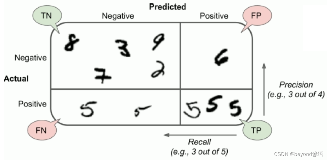
以MNIST手寫數字識別數據集為例，其對于的混淆矩陣如圖：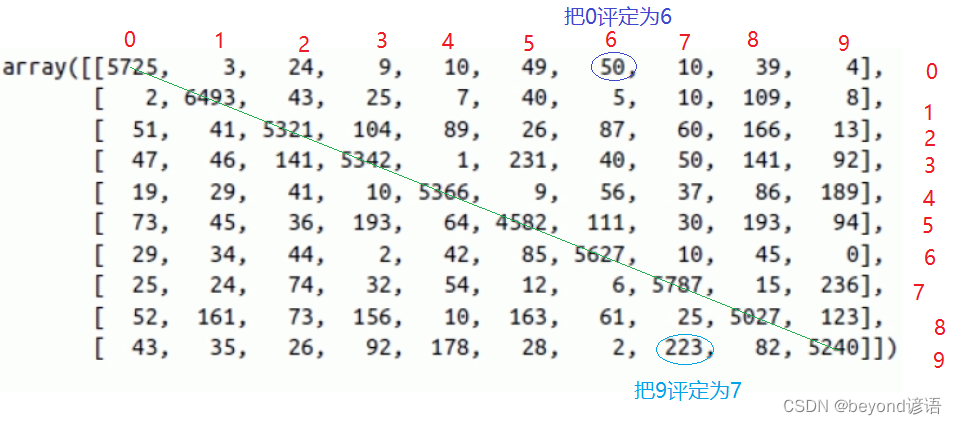
當然，對角線上的數值比較大，也就是判斷正確樣本數

五、準確率、召回率

P：你認為的是正例
N：你認為的是負例
例如：你要找全班的女生，此時男生就成為了負例，相應的女生就成為了正例。
T：判斷正確
F：判斷錯誤
判斷正確很好理解，人家是男生，你判斷成為了男生，那就是T；你判斷成了女生，那就是F。
TP：你認為是正例(P)，最后實際上這個就是正例，判斷正確(T)。一個人，你覺得人家是女生，實際上人家就是個女生，判斷正確，這就是TP。
FP：你認為是正例(P)，最后實際上這個卻是負例，判斷錯誤(F)。一個人，你覺得人家是女生，但實際上人家是個男生，判斷錯誤，這就是FP。
TN：你認為是負例(N)，最后實際上這個就是負例，判斷正確(T)。一個人，你覺得人家是男生，實際上人家就是個男生，判斷正確，這就是TN。
FN：你認為是負例(N)，最后實際上這個卻是負例，判斷錯誤(T)。一個人，你覺得人家是男生，但實際上人家是個女生，判斷錯誤，這就是FN。

Ⅰ，準確率

準確率：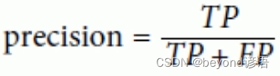
準確率更看重正例的表現
準確率就是在你認為是正確的樣例中，真正判斷對的有多少
例如：某購物軟件給二狗子推薦了10種商品(系統認為這是二狗子喜歡的東西)，但二狗子就選了3個點(實際上二狗子真正喜歡的東西)進去看了看。此時的準確率就是3/10=30%
隨著系統推薦的商品越來越多，準確率是下降的，因為分母是在變大。這就相當于言多必失！

Ⅱ，召回率

召回率：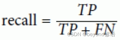
召回率也就是從真正正確的樣例中，召回了多少
例如：某購物軟件給二狗子推薦了10種商品(系統認為這是二狗子喜歡的東西)，但二狗子就選了3個點(實際上二狗子真正喜歡的東西)進去看了看，二狗子實際上真正喜歡1000種商品(真正的正確樣例)，也就是系統僅僅從二狗子喜歡的1000種商品中推選了3個給他。此時的召回率就是3/1000=0.3%
隨著系統推薦的商品越來越多，召回率是上升的，因為用戶喜歡的商品的總數是不變的，分母不變，推薦的越多越容易出現用戶喜歡的商品，也就是分子會越大。

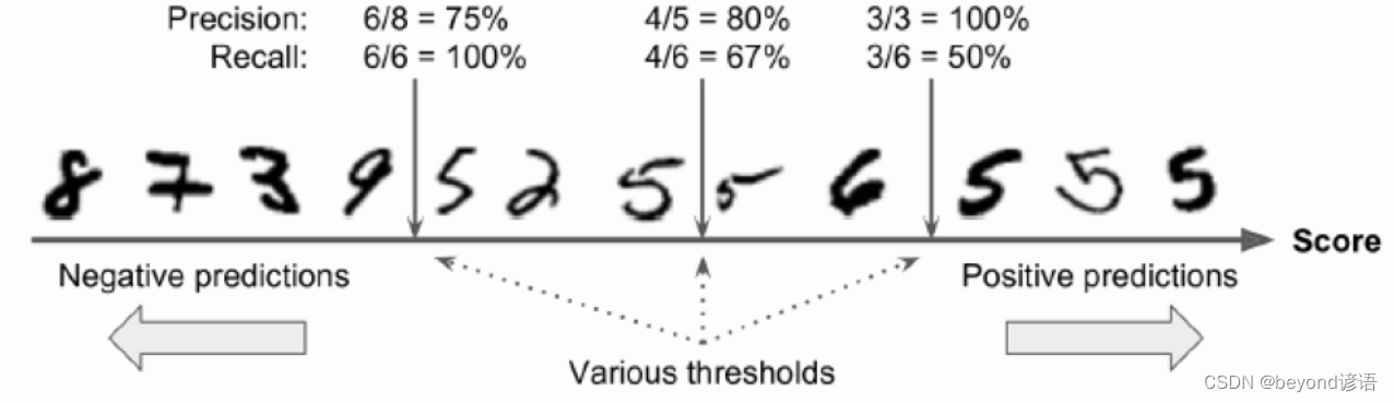
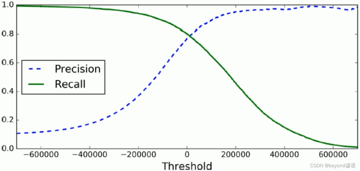
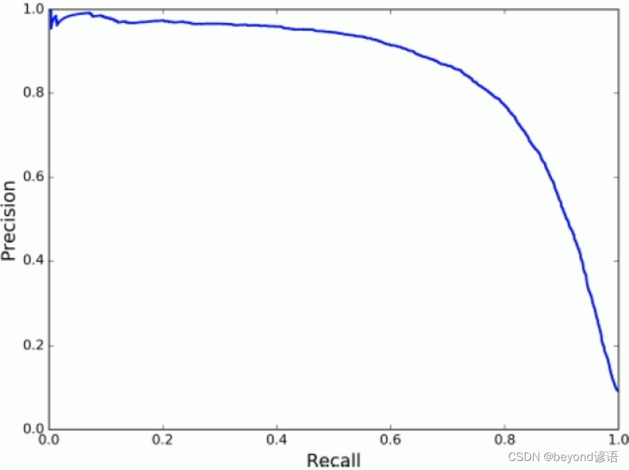
很顯然，準確率和召回率是相互抑制的關系，根據需要選擇其中一個指標作為核心，進行著重優化考慮，魚和熊掌不可兼得。
例如：給未成年人推薦視頻，寧可拒絕很多好的視頻，也不能推薦一個不良視頻，此時，就得使用低召回率，也就是要提高準確率。
監控畫面抓小偷，寧可把很多人都設成嫌疑犯，寧可工作量大一點，也不能錯過一個，也就是所謂的寧可錯殺一千也不放過一個，此時就需要高召回率，也就是要低準確率。

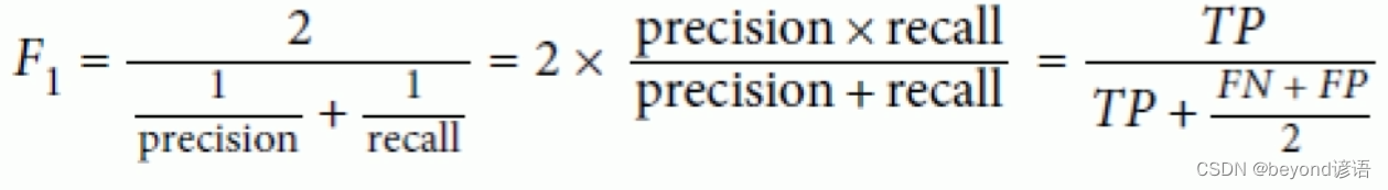
六、F1-Score(F1-Measure)

一個模型的好壞，單從準確率或者召回率看很顯然是不夠全面的，此時就出現了F1-Score，也稱F1-Measure。

七、TradeOff

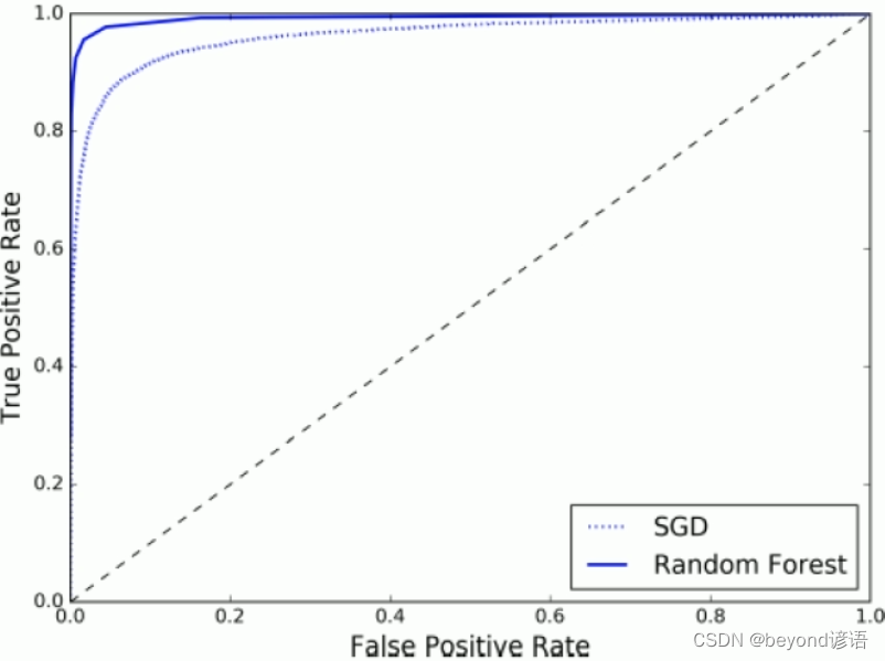
八、ROC曲線(Receiver Characteristic Operator)

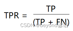，即所有正例中被正確的判定為正例的比例
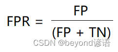，即所有負例中被錯誤的評定為正例的比例

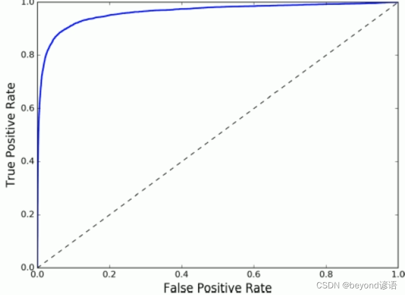
九、AUC面積(Area under Curve曲線下面積)

十、代碼實現

from sklearn.datasets import fetch_mldata
import matplotlib
import matplotlib.pyplot as plt
import numpy as np
from sklearn.linear_model import SGDClassifier
from sklearn.model_selection import StratifiedKFold
from sklearn.base import clone
from sklearn.model_selection import cross_val_score
from sklearn.base import BaseEstimator
from sklearn.model_selection import cross_val_predict
from sklearn.metrics import confusion_matrix
from sklearn.metrics import precision_score
from sklearn.metrics import recall_score
from sklearn.metrics import f1_score
from sklearn.metrics import precision_recall_curve
from sklearn.metrics import roc_curve
from sklearn.metrics import roc_auc_score
from sklearn.ensemble import RandomForestClassifiermnist = fetch_mldata('MNIST original', data_home='test_data_home')
print(mnist)
"""
{'DESCR': 'mldata.org dataset: mnist-original', 'COL_NAMES': ['label', 'data'], 'target': array([0., 0., 0., ..., 9., 9., 9.]), 'data': array([[0, 0, 0, ..., 0, 0, 0],[0, 0, 0, ..., 0, 0, 0],[0, 0, 0, ..., 0, 0, 0],...,[0, 0, 0, ..., 0, 0, 0],[0, 0, 0, ..., 0, 0, 0],[0, 0, 0, ..., 0, 0, 0]], dtype=uint8)}
"""X, y = mnist['data'], mnist['target']
print(X.shape, y.shape)
"""
(70000, 784) (70000,)
"""some_digit = X[36000]
print(some_digit)
some_digit_image = some_digit.reshape(28,28)
print(some_digit_image)#?(28,28)???????
# plt.imshow(some_digit_image, cmap=matplotlib.cm.binary,
#            interpolation='nearest')
# plt.axis('off')
# plt.show()#??60000??????????
X_train, X_test, y_train, y_test = X[:60000], X[60000:], y[:60000], y[:60000]
shuffle_index = np.random.permutation(60000)
X_train, y_train = X_train[shuffle_index], y_train[shuffle_index]y_train_5 = (y_train == 5)
y_test_5 = (y_test == 5)
print(y_test_5)
"""
[False False False ... False False False]
"""sgd_clf = SGDClassifier(loss='log', random_state=42,max_iter=500)
sgd_clf.fit(X_train, y_train_5)
print(sgd_clf.predict([some_digit]))
"""
[ True]
"""# skfolds = StratifiedKFold(n_splits=3, random_state=42)
#
# for train_index, test_index in skfolds.split(X_train, y_train_5):
#     clone_clf = clone(sgd_clf)
#     X_train_folds = X_train[train_index]
#     y_train_folds = y_train_5[train_index]
#     X_test_folds = X_train[test_index]
#     y_test_folds = y_train_5[test_index]
#
#     clone_clf.fit(X_train_folds, y_train_folds)
#     y_pred = clone_clf.predict(X_test_folds)
#     print(y_pred)
#     n_correct = sum(y_pred == y_test_folds)
#     print(n_correct / len(y_pred))'''
print(cross_val_score(sgd_clf, X_train, y_train_5, cv=3, scoring='accuracy'))
"""
[0.91185 0.95395 0.9641 ]
"""
print(cross_val_score(sgd_clf, X_train, y_train_5, cv=3, scoring='precision'))
"""
[0.50661455 0.69741533 0.81972989]
"""
'''# class Never5Classifier(BaseEstimator):
#     def fit(self, X, y=None):
#         pass
#
#     def predict(self, X):
#         return np.zeros((len(X), 1), dtype=bool)
#
#
# never_5_clf = Never5Classifier()
# print(cross_val_score(never_5_clf, X_train, y_train_5, cv=3, scoring='accuracy'))
# """
# [0.9098  0.9094  0.90975]
# """y_train_pred = cross_val_predict(sgd_clf, X_train, y_train_5, cv=3)
print(confusion_matrix(y_train_5, y_train_pred))
"""
[[53553  1026][ 1737  3684]]
"""y_train_perfect_prediction = y_train_5
print(confusion_matrix(y_train_5, y_train_perfect_prediction))
"""
[[54579     0][    0  5421]]
"""print(precision_score(y_train_5, y_train_pred))
print(recall_score(y_train_5, y_train_pred))
print(sum(y_train_pred))
print(f1_score(y_train_5, y_train_pred))
"""
0.7821656050955414
0.679579413392363
4710
0.7272727272727272
"""sgd_clf.fit(X_train, y_train_5)
y_scores = sgd_clf.decision_function([some_digit])
print(y_scores)threshold = 0
y_some_digit_pred = (y_scores > threshold)
print(y_some_digit_pred)threshold = 200000
y_some_digit_pred = (y_scores > threshold)
print(y_some_digit_pred)y_scores = cross_val_predict(sgd_clf, X_train, y_train_5, cv=3, method='decision_function')
print(y_scores)precisions, recalls, thresholds = precision_recall_curve(y_train_5, y_scores)
print(precisions, recalls, thresholds)def plot_precision_recall_vs_threshold(precisions, recalls, thresholds):plt.plot(thresholds, precisions[:-1], 'b--', label='Precision')plt.plot(thresholds, recalls[:-1], 'r--', label='Recall')plt.xlabel("Threshold")plt.legend(loc='upper left')plt.ylim([0, 1])plot_precision_recall_vs_threshold(precisions, recalls, thresholds)
plt.show()y_train_pred_90 = (y_scores > 70000)
print(precision_score(y_train_5, y_train_pred_90))
print(recall_score(y_train_5, y_train_pred_90))fpr, tpr, thresholds = roc_curve(y_train_5, y_scores)def plot_roc_curve(fpr, tpr, label=None):plt.plot(fpr, tpr, linewidth=2, label=label)plt.plot([0, 1], [0, 1], 'k--')plt.axis([0, 1, 0, 1])plt.xlabel('False Positive Rate')plt.ylabel('True positive Rate')plot_roc_curve(fpr, tpr)
plt.show()print(roc_auc_score(y_train_5, y_scores))forest_clf = RandomForestClassifier(random_state=42)
y_probas_forest = cross_val_predict(forest_clf, X_train, y_train_5, cv=3, method='predict_proba')
y_scores_forest = y_probas_forest[:, 1]fpr_forest, tpr_forest, thresholds_forest = roc_curve(y_train_5, y_scores_forest)
plt.plot(fpr, tpr, 'b:', label='SGD')
plt.plot(fpr_forest, tpr_forest, label='Random Forest')
plt.legend(loc='lower right')
plt.show()print(roc_auc_score(y_train_5, y_scores_forest))