文 /??李錫涵,Google Developers Expert
本文節選自《簡單粗暴 TensorFlow 2.0》

盡管 TensorFlow 2 建議以即時執行模式(Eager Execution)作為主要執行模式,然而,圖執行模式(Graph Execution)作為 TensorFlow 2 之前的主要執行模式,依舊對于我們理解 TensorFlow 具有重要意義。尤其是當我們需要使用 tf.function 時,對圖執行模式的理解更是不可或缺。
圖執行模式在 TensorFlow 1.X 和 2.X 版本中的 API 不同:- 在 TensorFlow 1.X 中,圖執行模式主要通過 “直接構建計算圖 +?
tf.Session” 進行操作; 在 TensorFlow 2 中,圖執行模式主要通過?
tf.function?進行操作。
提示
TensorFlow 2 依然支持 TensorFlow 1.X 的 API。為了在 TensorFlow 2 中使用 TensorFlow 1.X 的 API ,我們可以使用?import tensorflow.compat.v1 as tf?導入 TensorFlow,并通過?tf.disable_eager_execution()?禁用默認的即時執行模式。
TensorFlow 1+1
TensorFlow 的圖執行模式是一個符號式的(基于計算圖的)計算框架。簡而言之,如果你需要進行一系列計算,則需要依次進行如下兩步:- 建立一個 “計算圖”,這個圖描述了如何將輸入數據通過一系列計算而得到輸出;
建立一個會話,并在會話中與計算圖進行交互,即向計算圖傳入計算所需的數據,并從計算圖中獲取結果。
這里以計算 1+1 作為 Hello World 的示例。以下代碼通過 TensorFlow 1.X 的圖執行模式 API 計算 1+1:
import tensorflow.compat.v1 as tf
tf.disable_eager_execution()

# 以下三行定義了一個簡單的“計算圖”
a = tf.constant(1)  # 定義一個常量張量(Tensor)
b = tf.constant(1)
c = a + b           # 等價于 c = tf.add(a, b),c是張量a和張量b通過 tf.add 這一操作(Operation)所形成的新張量
# 到此為止,計算圖定義完畢,然而程序還沒有進行任何實質計算。
# 如果此時直接輸出張量 c 的值,是無法獲得 c = 2 的結果的

sess = tf.Session()     # 實例化一個會話(Session)
c_ = sess.run(c)        # 通過會話的 run() 方法對計算圖里的節點(張量)進行實際的計算
print(c_)
2
@tf.function修飾符對函數進行修飾。當需要運行此計算圖時,只需調用修飾后的函數即可。由此,我們可以將以上代碼改寫如下:import tensorflow as tf# 以下被 @tf.function 修飾的函數定義了一個計算圖@tf.functiondef graph():
a = tf.constant(1)
b = tf.constant(1)
c = a + breturn c# 到此為止,計算圖定義完畢。由于 graph() 是一個函數,在其被調用之前,程序是不會進行任何實質計算的。# 只有調用函數,才能通過函數返回值,獲得 c = 2 的結果
c_ = graph()
print(c_.numpy())
計算圖中的占位符與數據輸入?小結
在 TensorFlow 1.X 的 API 中,我們直接在主程序中建立計算圖。而在 TensorFlow 2 中,計算圖的建立需要被封裝在一個被
@tf.function修飾的函數中;在 TensorFlow 1.X 的 API 中,我們通過實例化一個
tf.Session,并使用其run方法執行計算圖的實際運算。而在 TensorFlow 2 中,我們通過直接調用被@tf.function修飾的函數來執行實際運算。
上面這個程序只能計算 1+1,以下代碼通過 TensorFlow 1.X 的圖執行模式 API 中的 tf.placeholder() (占位符張量)和 sess.run() 的 feed_dict 參數,展示了如何使用 TensorFlow 計算任意兩個數的和:
import tensorflow.compat.v1 as tf
tf.disable_eager_execution()

a = tf.placeholder(dtype=tf.int32)  # 定義一個占位符Tensor
b = tf.placeholder(dtype=tf.int32)
c = a + b

a_ = int(input("a = "))  # 從終端讀入一個整數并放入變量a_
b_ = int(input("b = "))

sess = tf.Session()
c_ = sess.run(c, feed_dict={a: a_, b: b_})  # feed_dict參數傳入為了計算c所需要的張量的值
print("a + b = %d" % c_)
運行程序:
>>> a = 2
>>> b = 3
a + b = 5
而在 TensorFlow 2 中,我們可以通過為函數指定參數來實現與占位符張量相同的功能。為了在計算圖運行時送入占位符數據,只需在調用被修飾后的函數時,將數據作為參數傳入即可。由此,我們可以將以上代碼改寫如下:
import tensorflow as tf

@tf.function
def graph(a, b):
    c = a + b
return c

a_ = int(input("a = "))
b_ = int(input("b = "))
c_ = graph(a_, b_)
print("a + b = %d" % c_)
計算圖中的變量?小結在 TensorFlow 1.X 的 API 中,我們使用
tf.placeholder()在計算圖中聲明占位符張量,并通過sess.run()的feed_dict參數向計算圖中的占位符傳入實際數據。而在 TensorFlow 2 中,我們使用tf.function的函數參數作為占位符張量,通過向被@tf.function修飾的函數傳遞參數,來為計算圖中的占位符張量提供實際數據。
變量的聲明?
變量(Variable)是一種特殊類型的張量,使用tf.get_variable()建立,與編程語言中的變量很相似。使用變量前需要先初始化,變量內存儲的值可以在計算圖的計算過程中被修改。以下示例代碼展示了如何建立一個變量,將其值初始化為 0,并逐次累加 1。import tensorflow.compat.v1 as tf
tf.disable_eager_execution()
a = tf.get_variable(name='a', shape=[])
initializer = tf.assign(a, 0.0) # tf.assign(x, y)返回一個“將張量y的值賦給變量x”的操作
plus_one_op = tf.assign(a, a + 1.0)
sess = tf.Session()
sess.run(initializer)
for i in range(5):
sess.run(plus_one_op) # 對變量a執行加一操作
print(sess.run(a)) # 輸出此時變量a在當前會話的計算圖中的值
1.0
2.0
3.0
4.0
5.0
在 TensorFlow 2 中,我們通過實例化提示為了初始化變量,也可以在聲明變量時指定初始化器(initializer),并通過
tf.global_variables_initializer()一次性初始化所有變量,在實際工程中更常用:import tensorflow.compat.v1 as tf
tf.disable_eager_execution()
a = tf.get_variable(name='a', shape=[],
initializer=tf.zeros_initializer) # 指定初始化器為全0初始化
plus_one_op = tf.assign(a, a + 1.0)
sess = tf.Session()
sess.run(tf.global_variables_initializer()) # 初始化所有變量
for i in range(5):
sess.run(plus_one_op)
print(sess.run(a)
tf.Variable類來聲明變量。由此,我們可以將以上代碼改寫如下:import tensorflow as tf
a = tf.Variable(0.0)
@tf.function
def plus_one_op():
a.assign(a + 1.0)
return a
for i in range(5):
plus_one_op()
print(a.numpy())
變量的作用域與重用?在 TensorFlow 1.X 中,我們建立模型時經常需要指定變量的作用域,以及復用變量。此時,TensorFlow 1.X 的圖執行模式 API 為我們提供了小結
在 TensorFlow 1.X 的 API 中,我們使用tf.get_variable()在計算圖中聲明變量節點。而在 TensorFlow 2 中,我們直接通過tf.Variable實例化變量對象,并在計算圖中使用這一變量對象。
tf.variable_scope() 及 reuse 參數來實現變量作用域和復用變量的功能。以下的例子使用了 TensorFlow 1.X 的圖執行模式 API 建立了一個三層的全連接神經網絡,其中第三層復用了第二層的變量。import tensorflow.compat.v1 as tf
import numpy as np
tf.disable_eager_execution()
def dense(inputs, num_units):
weight = tf.get_variable(name='weight', shape=[inputs.shape[1], num_units])
bias = tf.get_variable(name='bias', shape=[num_units])
return tf.nn.relu(tf.matmul(inputs, weight) + bias)
def model(inputs):
with tf.variable_scope('dense1'): # 限定變量的作用域為 dense1
x = dense(inputs, 10) # 聲明了 dense1/weight 和 dense1/bias 兩個變量
with tf.variable_scope('dense2'): # 限定變量的作用域為 dense2
x = dense(x, 10) # 聲明了 dense2/weight 和 dense2/bias 兩個變量
with tf.variable_scope('dense2', reuse=True): # 第三層復用第二層的變量
x = dense(x, 10)
return x
inputs = tf.placeholder(shape=[10, 32], dtype=tf.float32)
outputs = model(inputs)
print(tf.global_variables()) # 輸出當前計算圖中的所有變量節點
sess = tf.Session()
sess.run(tf.global_variables_initializer())
outputs_ = sess.run(outputs, feed_dict={inputs: np.random.rand(10, 32)})
print(outputs_)
['dense1/weight:0' shape=(32, 10) dtype=float32>,'dense1/bias:0' shape=(10,) dtype=float32>,'dense2/weight:0' shape=(10, 10) dtype=float32>,'dense2/bias:0' shape=(10,) dtype=float32>]可見,tf.variable_scope() 為在其上下文中的,以 tf.get_variable 建立的變量的名稱添加了 “前綴” 或 “作用域”,使得變量在計算圖中的層次結構更為清晰,不同 “作用域” 下的同名變量各司其職,不會沖突。同時,雖然我們在上例中調用了 3 次 dense 函數,即調用了 6 次 tf.get_variable 函數,但實際建立的變量節點只有 4 個。這即是 tf.variable_scope() 的 reuse 參數所起到的作用。當 reuse=True 時, tf.get_variable 遇到重名變量時將會自動獲取先前建立的同名變量,而不會新建變量,從而達到了變量重用的目的。
tf.variable_scope() ,而應當使用 tf.keras.layers.Layer 和 tf.keras.Model 來封裝代碼和指定作用域,具體可參考 本手冊第三章。上面的例子與下面基于 tf.keras 和 tf.function 的代碼等價。import tensorflow as tf
import numpy as np
class Dense(tf.keras.layers.Layer):
def __init__(self, num_units, **kwargs):
super().__init__(**kwargs)
self.num_units = num_units
def build(self, input_shape):
self.weight = self.add_variable(name='weight', shape=[input_shape[-1], self.num_units])
self.bias = self.add_variable(name='bias', shape=[self.num_units])
def call(self, inputs):
y_pred = tf.matmul(inputs, self.weight) + self.bias
return y_pred
class Model(tf.keras.Model):
def __init__(self):
super().__init__()
self.dense1 = Dense(num_units=10, name='dense1')
self.dense2 = Dense(num_units=10, name='dense2')
@tf.function
def call(self, inputs):
x = self.dense1(inputs)
x = self.dense2(inputs)
x = self.dense2(inputs)
return x
model = Model()
print(model(np.random.rand(10, 32)))
我們可以注意到,在 TensorFlow 2 中,變量的作用域以及復用變量的問題自然地淡化了。基于 Python 類的模型建立方式自然地為變量指定了作用域,而變量的重用也可以通過簡單地多次調用同一個層來實現。
為了詳細了解上面的代碼對變量作用域的處理方式,我們使用get_concrete_function導出計算圖,并輸出計算圖中的所有變量節點:graph = model.call.get_concrete_function(np.random.rand(10, 32))
print(graph.variables)
('dense1/weight:0' shape=(32, 10) dtype=float32, numpy=...>,'dense1/bias:0' shape=(10,) dtype=float32, numpy=...>,'dense2/weight:0' shape=(32, 10) dtype=float32, numpy=...>,'dense2/bias:0' shape=(10,) dtype=float32, numpy=...)name參數為每個層指定的名稱將成為層內變量的作用域。小結
在 TensorFlow 1.X 的 API 中,使用tf.variable_scope()及reuse參數來實現變量作用域和復用變量的功能。在 TensorFlow 2 中,使用tf.keras.layers.Layer和tf.keras.Model來封裝代碼和指定作用域,從而使變量的作用域以及復用變量的問題自然淡化。兩者的實質是一樣的。
自動求導機制與優化器?
在本節中,我們對 TensorFlow 1.X 和 TensorFlow 2 在圖執行模式下的自動求導機制進行較深入的比較說明。
自動求導機制?我們首先回顧 TensorFlow 1.X 中的自動求導機制。在 TensorFlow 1.X 的圖執行模式 API 中,可以使用tf.gradients(y, x) 計算計算圖中的張量節點 y 相對于變量 x 的導數。以下示例展示了在 TensorFlow 1.X 的圖執行模式 API 中計算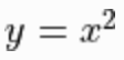 在
在 時的導數。
時的導數。x = tf.get_variable('x', dtype=tf.float32, shape=[], initializer=tf.constant_initializer(3.))
y = tf.square(x) # y = x ^ 2
y_grad = tf.gradients(y, x)以上代碼中,計算圖中的節點 y_grad 即為 y 相對于 x 的導數。
而在 TensorFlow 2 的圖執行模式 API 中,我們使用 tf.GradientTape 這一上下文管理器封裝需要求導的計算步驟,并使用其 gradient 方法求導,代碼示例如下:
x = tf.Variable(3.)
@tf.function
def grad():
with tf.GradientTape() as tape:
        y = tf.square(x)
    y_grad = tape.gradient(y, x)
return y_grad
優化器小結
在 TensorFlow 1.X 中,我們使用tf.gradients()求導。而在 TensorFlow 2 中,我們使用使用tf.GradientTape這一上下文管理器封裝需要求導的計算步驟,并使用其gradient方法求導。
由于機器學習中的求導往往伴隨著優化,所以 TensorFlow 中更常用的是優化器(Optimizer)。在 TensorFlow 1.X 的圖執行模式 API 中,我們往往使用tf.train中的各種優化器,將求導和調整變量值的步驟合二為一。例如,以下代碼片段在計算圖構建過程中,使用 tf.train.GradientDescentOptimizer這一梯度下降優化器優化損失函數 loss :
y_pred = model(data_placeholder)    # 模型構建
loss = ...                          # 計算模型的損失函數 loss
optimizer = tf.train.GradientDescentOptimizer(learning_rate=0.001)
train_one_step = optimizer.minimize(loss)
# 上面一步也可拆分為
# grad = optimizer.compute_gradients(loss)
# train_one_step = optimizer.apply_gradients(grad)
以上代碼中, train_one_step 即為一個將求導和變量值更新合二為一的計算圖節點(操作),也就是訓練過程中的 “一步”。特別需要注意的是,對于優化器的 minimize 方法而言,只需要指定待優化的損失函數張量節點 loss 即可,求導的變量可以自動從計算圖中獲得(即 tf.trainable_variables )。在計算圖構建完成后,只需啟動會話,使用 sess.run 方法運行 train_one_step 這一計算圖節點,并通過 feed_dict 參數送入訓練數據,即可完成一步訓練。代碼片段如下:
for data in dataset:
    data_dict = ... # 將訓練所需數據放入字典 data 內
    sess.run(train_one_step, feed_dict=data_dict)
而在 TensorFlow 2 的 API 中,無論是圖執行模式還是即時執行模式,均先使用 tf.GradientTape 進行求導操作,然后再使用優化器的 apply_gradients 方法應用已求得的導數,進行變量值的更新。也就是說,和 TensorFlow 1.X 中優化器的 compute_gradients + apply_gradients 十分類似。同時,在 TensorFlow 2 中,無論是求導還是使用導數更新變量值,都需要顯式地指定變量。計算圖的構建代碼結構如下:
optimizer = tf.keras.optimizer.SGD(learning_rate=...)

@tf.function
def train_one_step(data):
with tf.GradientTape() as tape:
        y_pred = model(data)    # 模型構建
        loss = ...              # 計算模型的損失函數 loss
    grad = tape.gradient(loss, model.variables)
optimizer.apply_gradients(grads_and_vars=zip(grads, model.variables))train_one_step函數并送入訓練數據即可:for data in dataset:
train_one_step(data)
自動求導機制的計算圖對比 *小結
在 TensorFlow 1.X 中,我們多使用優化器的minimize方法,將求導和變量值更新合二為一。而在 TensorFlow 2 中,我們需要先使用tf.GradientTape進行求導操作,然后再使用優化器的apply_gradients方法應用已求得的導數,進行變量值的更新。而且在這兩步中,都需要顯式指定待求導和待更新的變量。
在本節,為了幫助讀者更深刻地理解 TensorFlow 的自動求導機制,我們以前節的 “計算??在?時的導數” 為例,展示 TensorFlow 1.X 和 TensorFlow 2 在圖執行模式下,為這一求導過程所建立的計算圖,并進行詳細講解。
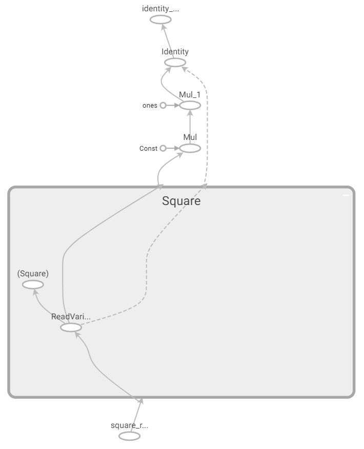
在 TensorFlow 1.X 的圖執行模式 API 中,將生成的計算圖使用 TensorBoard 進行展示:
 在計算圖中,灰色的塊為節點的命名空間(Namespace,后文簡稱 “塊”),橢圓形代表操作節點(OpNode),圓形代表常量,灰色的箭頭代表數據流。為了弄清計算圖節點
 x 、 y 和 y_grad 與計算圖中節點的對應關系,我們將這些變量節點輸出,可見:x:?y:Tensor("Square:0", shape=(), dtype=float32)y_grad:[]
在 TensorBoard 中,我們也可以通過點擊節點獲得節點名稱。通過比較我們可以得知,變量 x 對應計算圖最下方的 x,節點 y 對應計算圖 “Square” 塊的 “ (Square) ”,節點 y_grad 對應計算圖上方 “Square_grad” 的 Mul_1 節點。同時我們還可以通過點擊節點發現,“Square_grad” 塊里的 const 節點值為 2,“gradients” 塊里的 grad_ys_0 值為 1, Shape 值為空,以及 “x” 塊的 const 節點值為 3。
接下來,我們開始具體分析這個計算圖的結構。我們可以注意到,這個計算圖的結構是比較清晰的,“x” 塊負責變量的讀取和初始化,“Square” 塊負責求平方 y = x ^ 2 ,而 “gradients” 塊則負責對 “Square” 塊的操作求導,即計算 y_grad = 2 * x。由此我們可以看出, tf.gradients 是一個相對比較 “龐大” 的操作,并非如一般的操作一樣往計算圖中添加了一個或幾個節點,而是建立了一個龐大的子圖,以應用鏈式法則求計算圖中特定節點的導數。
在 TensorFlow 2 的圖執行模式 API 中,將生成的計算圖使用 TensorBoard 進行展示:
 我們可以注意到,除了求導過程沒有封裝在 “gradients” 塊內,以及變量的處理簡化以外,其他的區別并不大。由此,我們可以看出,在圖執行模式下,
 tf.GradientTape這一上下文管理器的 gradient 方法和 TensorFlow 1.X 的 tf.gradients 是基本等價的。小結
TensorFlow 1.X 中的tf.gradients和 TensorFlow 2 圖執行模式下的tf.GradientTape上下文管理器盡管在 API 層面的調用方法略有不同,但最終生成的計算圖是基本一致的。


“哪吒頭”—玩轉小潮流


 - 整體執行流程分析)

自動化測試教程(10) 使用 Jenkins 構建自動化測試持續集成...)


)


