一、為什么是灰度圖

相較于 RGB 三通道圖像，灰度圖僅保留亮度信息（Y 分量），數據量減少 2/3，相比于常用的 NV12 圖像，數據量減少 1/3，內存占用與計算負載顯著降低。對于下游網絡結構而言，單通道網絡計算量/參數量也會更少，這對邊緣設備的實時處理至關重要。

灰度圖部署有一個問題：如何將視頻流中的 NV12 數據高效轉換為模型所需的灰度輸入，并在工具鏈中實現標準化前處理流程。

視頻通路傳輸的原始數據通常采用 NV12 格式，這是一種適用于 YUV 色彩空間的半平面格式：

• 數據結構：NV12 包含一個平面的 Y 分量（亮度信息）和一個平面的 UV 分量（色度信息），其中 Y 分量分辨率為 W×H，UV 分量分辨率為 W×H/2。
• 灰度圖提取：對于灰度圖部署，僅需使用 NV12 中的 Y 分量。以 1920×1080 分辨率為例，若 NV12 中 Y 與 UV 分量連續存儲，Y 分量占據前 1920×1080 字節，后續部分為 UV 分量，可直接忽略或舍棄，若分開存儲，使用起來更簡單。

二、灰度圖部署數據鏈路

視頻通路過來的數據不能直接是灰度圖，而是 nv12 數據，對于灰度圖部署，可以只使用其中的 y 分量。

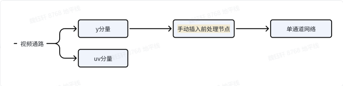
2.1 手動插入前處理節點

在工具鏈提供的絕大部分材料中，前處理節點多是對于 3 通道網絡、nv12 輸入進行的，查看工具鏈用戶手冊《進階內容->HBDK Tool API Reference》中幾處 api 介紹，可以發現也是支持 gray 灰度圖的，具體內容如下：

• insert_image_convert(self, mode str = “nv12”)

Insert image_convert op. Change input parameter type.Args:* mode (str): Specify conversion mode, optional values are "nv12"(default) and "gray".Returns:List of newly inserted function arguments which is also the inputs of inserted image convert opRaises:ValueError when this argument is no longer validNote:To avoid the new insertion operator not running in some conversion passes, it is recommended to call the insert_xxx api before the convert stageExample:module = load("model.bc")func = module[0]res = func.inputs[0].insert_image_convert("nv12")

對于 batch 輸入，均值、標準化、歸一化等操作，可以在 insert_image_preprocess 中實現：

• insert_image_preprocess( self, mode str, divisor int, mean List[float], std List[float], is_signed bool = True)

Insert image_convert op. Change input parameter type.Args:* mode (str): Specify conversion mode, optional values are "skip"(default, same as None), "yuvbt601full2rgb", "yuvbt601full2bgr", "yuvbt601video2rgb" and "yuvbt601video2bgr".Returns:List of newly inserted function arguments which is also the inputs of inserted image preprocess opRaises:ValueError when this argument is no longer validNote:To avoid the new insertion operator not running in some conversion passes, it is recommended to call the insert_xxx api before the convert stageExample:module = load("model.bc")func = module[0]res = func.inputs[0].insert_image_preprocess("yuvbt601full2rgb", 255, [0.485, 0.456, 0.406], [0.229, 0.224, 0.225], True)

手動插入前處理節點可參考：

mean = [0.485]
std = [0.229]
func = qat_bc[0]for input in func.flatten_inputs[::-1]:split_inputs = input.insert_split(dim=0)for split_input in reversed(split_inputs):node = split_input.insert_transpose([0, 3, 1, 2])node = node.insert_image_preprocess(mode="skip",divisor=255,mean=mean,std=std,is_signed=True)node.insert_image_convert(mode="gray")

• mean = [0.485] 和 std = [0.229]：定義圖像歸一化時使用的均值和標準差
• func = qat_bc[0]：獲取量化感知訓練 （QAT） 模型中的第一個函數 / 模塊作為處理入口。
• for input in func.flatten_inputs[::-1]：逆序遍歷模型的所有扁平化輸入節點。
• split_inputs = input.insert_split（dim=0）：將輸入數據按批次維度 （dim=0） 分割，這是處理 batch 輸入必須要做的。
• node = split_input.insert_transpose（[0， 3， 1， 2]）：將數據維度從[B， H， W， C]（NHWC 格式） 轉換為[B， C， H， W]（NCHW 格式），也是必須要做的。
• node.insert_image_preprocess（…）：執行圖像預處理
• node.insert_image_convert（mode=“gray”）：插入單通道灰度圖

三、全流程示例代碼

import torch
import torch.nn as nn
import torch.nn.functional as F
from horizon_plugin_pytorch import set_march, March
set_march(March.NASH_M)
from horizon_plugin_pytorch.quantization import prepare, set_fake_quantize, FakeQuantState
from horizon_plugin_pytorch.quantization import QuantStub
from horizon_plugin_pytorch.quantization.hbdk4 import export
from horizon_plugin_pytorch.quantization.qconfig_template import calibration_8bit_weight_16bit_act_qconfig_setter, default_calibration_qconfig_setter
from horizon_plugin_pytorch.quantization.qconfig import get_qconfig, MSEObserver, MinMaxObserver
from horizon_plugin_pytorch.dtype import qint8, qint16
from torch.quantization import DeQuantStub
from hbdk4.compiler import statistics, save, load,visualize,compile,convert, hbm_perfclass SimpleConvNet(nn.Module):def __init__(self):super(SimpleConvNet, self).__init__()# 第一個節點：輸入通道 1，輸出通道 16，卷積核 3x3self.conv1 = nn.Conv2d(in_channels=1, out_channels=16, kernel_size=3, stride=1, padding=1)# 后續添加一個池化層和一個全連接層self.pool = nn.MaxPool2d(kernel_size=2, stride=2)self.fc = nn.Linear(16 * 14 * 14, 10)  # 假設輸入圖像為 28x28self.quant = QuantStub()self.dequant = DeQuantStub()def forward(self, x):x = self.quant(x)x = self.conv1(x)      # 卷積層x = F.relu(x)          # 激活x = self.pool(x)       # 池化x = x.view(x.size(0), -1)  # Flattenx = self.fc(x)         # 全連接層輸出x = self.dequant(x)return x# 構造模型
model = SimpleConvNet()# 構造一個假輸入：batch_size=4，單通道，28x28 圖像
example_input = torch.randn(4, 1, 28, 28)
output = model(example_input)print("輸出 shape:", output.shape)  # torch.Size([4, 10])calib_model = prepare(model.eval(), example_input, qconfig_setter=(default_calibration_qconfig_setter,),)calib_model.eval()
set_fake_quantize(calib_model, FakeQuantState.CALIBRATION)
calib_model(example_input)calib_model.eval()                            
set_fake_quantize(calib_model, FakeQuantState.VALIDATION)
calib_out = calib_model(example_input)
print("calib輸出數據:", calib_out)qat_bc = export(calib_model, example_input)
mean = [0.485]
std = [0.229]
func = qat_bc[0]for input in func.flatten_inputs[::-1]:split_inputs = input.insert_split(dim=0)for split_input in reversed(split_inputs):node = split_input.insert_transpose([0, 3, 1, 2])node = node.insert_image_preprocess(mode="skip",divisor=255,mean=mean,std=std,is_signed=True)node.insert_image_convert(mode="gray")quantized_bc = convert(qat_bc, "nash-m")
hbir_func = quantized_bc.functions[0]
hbir_func.remove_io_op(op_types = ["Dequantize","Quantize"])
visualize(quantized_bc, "model_result/quantized_batch4.onnx")
statistics(quantized_bc)
params = {'jobs': 64, 'balance': 100, 'progress_bar': True,'opt': 2,'debug': True, "advice": 0.0}
hbm_path="model_result/batch4-gray.hbm"
print("start to compile")
compile(quantized_bc, march="nash-m", path=hbm_path, **params)
print("end to compile")
ebug': True, "advice": 0.0}
hbm_path="model_result/batch4-gray.hbm"
print("start to compile")
compile(quantized_bc, march="nash-m", path=hbm_path, **params)
print("end to compile")