使用決策樹訓練紅酒數據集
完整代碼:
import numpy as np
import matplotlib.pyplot as plt
from matplotlib.colors import ListedColormap
from sklearn import tree, datasets
from sklearn.model_selection import train_test_split# 準備數據,這里使用前兩個特征
data = datasets.load_wine()
X, y = data.data[:,:2], data.target
X_train, X_test, y_train, y_test = train_test_split(X, y)# 訓練模型
clf = tree.DecisionTreeClassifier(max_depth=1)
clf.fit(X, y)print(clf.score(X_test, y_test))
輸出:
0.7555555555555555
繪制決策樹的圖形
完整代碼:
import numpy as np
import matplotlib.pyplot as plt
from matplotlib.colors import ListedColormap
from sklearn import tree, datasets
from sklearn.model_selection import train_test_split# 準備數據,這里使用前兩個特征
data = datasets.load_wine()
X, y = data.data[:,:2], data.target
X_train, X_test, y_train, y_test = train_test_split(X, y)# 訓練模型
clf = tree.DecisionTreeClassifier(max_depth=1)
clf.fit(X, y)# 畫圖
cmap_light = ListedColormap(["#FFAAAA", "#AAFFAA", "#AAAAFF"])
cmap_bold = ListedColormap(["#FF0000", "#00FF00", "#0000FF"])x_min, x_max = X_train[:,0].min() - 1, X_train[:,0].max() + 1
y_min, y_max = X_train[:,1].min() - 1, X_train[:,1].max() + 1
xx, yy = np.meshgrid(np.arange(x_min, x_max, .02), np.arange(y_min, y_max, .02))
z = clf.predict(np.c_[xx.ravel(), yy.ravel()]).reshape(xx.shape)plt.figure()
plt.pcolormesh(xx, yy, z, cmap=cmap_light)plt.scatter(X[:, 0], X[:, 1], c=y, cmap=cmap_bold, edgecolor="k", s=20)
plt.xlim(xx.min(), xx.max())
plt.ylim(yy.min(), yy.max())
plt.title("Classifier: (max_depth = 1)")
plt.show()
輸出:
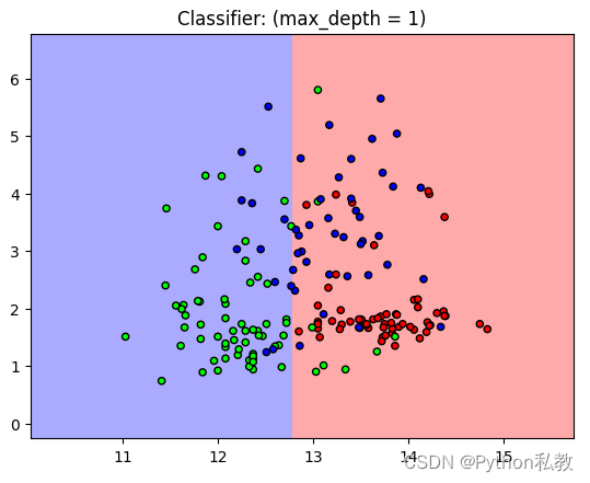
從結果來看,分類器的表現并不是特別好,我們可以加大深度試試。
調整決策樹的深度
完整代碼:
import numpy as np
import matplotlib.pyplot as plt
from matplotlib.colors import ListedColormap
from sklearn import tree, datasets
from sklearn.model_selection import train_test_split# 準備數據,這里使用前兩個特征
data = datasets.load_wine()
X, y = data.data[:,:2], data.target
X_train, X_test, y_train, y_test = train_test_split(X, y)# 訓練模型
clf = tree.DecisionTreeClassifier(max_depth=3)
clf.fit(X, y)
print(clf.score(X_test, y_test))# 畫圖
cmap_light = ListedColormap(["#FFAAAA", "#AAFFAA", "#AAAAFF"])
cmap_bold = ListedColormap(["#FF0000", "#00FF00", "#0000FF"])x_min, x_max = X_train[:,0].min() - 1, X_train[:,0].max() + 1
y_min, y_max = X_train[:,1].min() - 1, X_train[:,1].max() + 1
xx, yy = np.meshgrid(np.arange(x_min, x_max, .02), np.arange(y_min, y_max, .02))
z = clf.predict(np.c_[xx.ravel(), yy.ravel()]).reshape(xx.shape)plt.figure()
plt.pcolormesh(xx, yy, z, cmap=cmap_light)plt.scatter(X[:, 0], X[:, 1], c=y, cmap=cmap_bold, edgecolor="k", s=20)
plt.xlim(xx.min(), xx.max())
plt.ylim(yy.min(), yy.max())
plt.title("Classifier: (max_depth = 3)")
plt.show()
輸出:
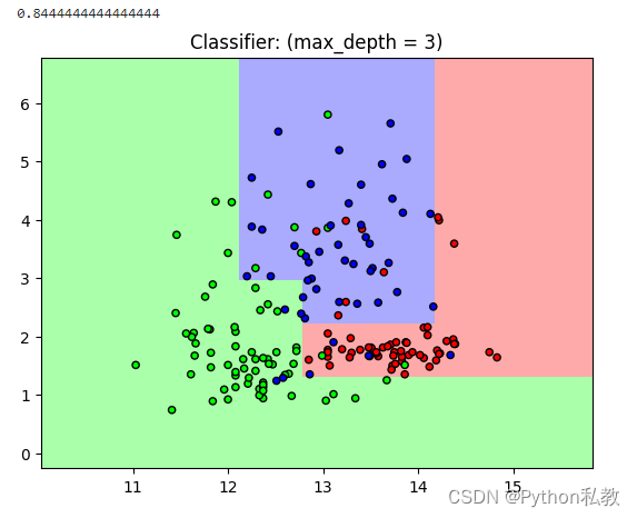
從結果來看,分數變成了0.84,已經是一個比較能夠接受的分數了。
另外,從圖像來看,不同的點大致都能落入到自己的區域中,相比深度為1的時候更加的準確一點。
繼續加大決策樹的深度
完整代碼:
import numpy as np
import matplotlib.pyplot as plt
from matplotlib.colors import ListedColormap
from sklearn import tree, datasets
from sklearn.model_selection import train_test_split# 準備數據,這里使用前兩個特征
data = datasets.load_wine()
X, y = data.data[:,:2], data.target
X_train, X_test, y_train, y_test = train_test_split(X, y)# 訓練模型
clf = tree.DecisionTreeClassifier(max_depth=5)
clf.fit(X, y)
print(clf.score(X_test, y_test))# 畫圖
cmap_light = ListedColormap(["#FFAAAA", "#AAFFAA", "#AAAAFF"])
cmap_bold = ListedColormap(["#FF0000", "#00FF00", "#0000FF"])x_min, x_max = X_train[:,0].min() - 1, X_train[:,0].max() + 1
y_min, y_max = X_train[:,1].min() - 1, X_train[:,1].max() + 1
xx, yy = np.meshgrid(np.arange(x_min, x_max, .02), np.arange(y_min, y_max, .02))
z = clf.predict(np.c_[xx.ravel(), yy.ravel()]).reshape(xx.shape)plt.figure()
plt.pcolormesh(xx, yy, z, cmap=cmap_light)plt.scatter(X[:, 0], X[:, 1], c=y, cmap=cmap_bold, edgecolor="k", s=20)
plt.xlim(xx.min(), xx.max())
plt.ylim(yy.min(), yy.max())
plt.title("Classifier: (max_depth = 5)")
plt.show()
輸出:
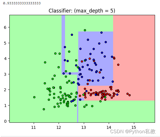
從結果來看,分數從0.84變成了0.93,明顯更加的準確了。


)
)


)


