文章目錄
- Biclustering (雙聚類)
- 譜二分聚類算法演示
- 生成樣本數據
- 擬合 `SpectralBiclustering`
- 繪制結果
- Spectral Co-Clustering 算法演示
- 使用光譜協同聚類算法進行文檔的二分聚類
Biclustering (雙聚類)
關于雙聚類技術的示例。
譜雙聚類的演示
譜雙聚類的演示
使用譜協同聚類算法對文檔進行雙聚類
使用譜協同聚類算法對文檔進行雙聚類

使用譜協同聚類算法對新聞組文檔進行雙聚類
使用譜協同聚類算法對新聞組文檔進行雙聚類
注意:前往末尾下載完整示例代碼或通過 JupyterLite 或 Binder 在瀏覽器中運行此示例。
譜二分聚類算法演示
本例演示了如何使用 SpectralBiclustering 算法生成方格數據集并對其進行二分聚類。譜二分聚類算法專門設計用于通過同時考慮矩陣的行(樣本)和列(特征)來聚類數據。它的目標是識別樣本之間以及樣本子集中的模式,從而在數據中檢測到局部化結構。這使得譜二分聚類特別適合于特征順序或排列固定的數據集,例如圖像、時間序列或基因組。
數據生成后,經過打亂并傳遞給譜二分聚類算法。然后重新排列打亂矩陣的行和列來繪制找到的二分聚類。
# 作者:scikit-learn 開發者
# SPDX-License-Identifier: BSD-3-Clause
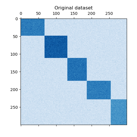
生成樣本數據
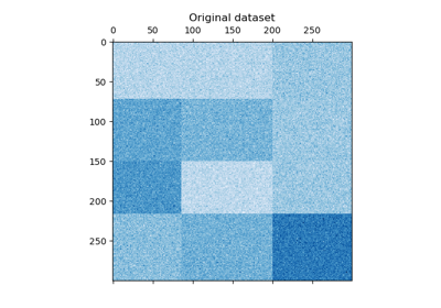
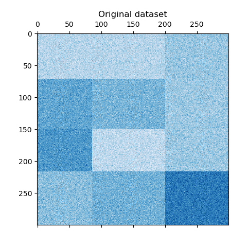
我們使用 make_checkerboard 函數生成樣本數據。shape=(300, 300) 中的每個像素都代表來自均勻分布的值。噪聲來自正態分布,其中 noise 的值是標準差。
如您所見,數據分布在 12 個簇單元中,且相對容易區分。
from matplotlib import pyplot as pltfrom sklearn.datasets import make_checkerboardn_clusters = (4, 3)
data, rows, columns = make_checkerboard(shape=(300, 300), n_clusters=n_clusters, noise=10, shuffle=False, random_state=42
)plt.matshow(data, cmap=plt.cm.Blues)
plt.title("原始數據集")
plt.show()
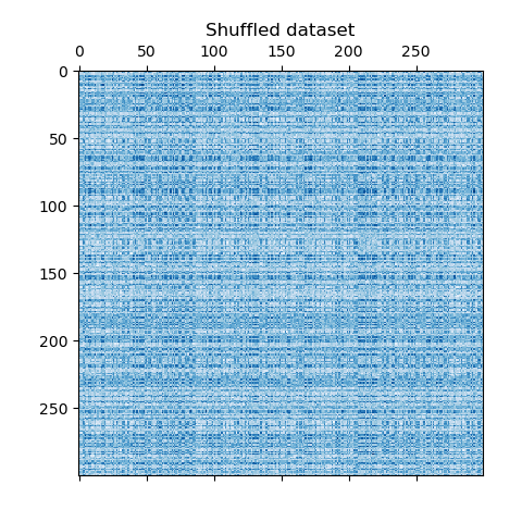
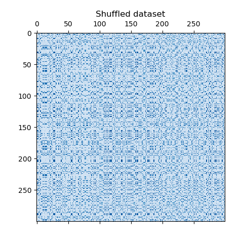
我們打亂數據,目標是之后使用 SpectralBiclustering 重建它。
import numpy as np# 創建打亂行和列索引的列表
rng = np.random.RandomState(0)
row_idx_shuffled = rng.permutation(data.shape[0])
col_idx_shuffled = rng.permutation(data.shape[1])
我們重新定義打亂的數據并繪制它。我們觀察到我們失去了原始數據矩陣的結構。
data = data[row_idx_shuffled][:, col_idx_shuffled]plt.matshow(data, cmap=plt.cm.Blues)
plt.title("打亂的數據集")
plt.show()
擬合 SpectralBiclustering
我們擬合模型并比較獲得的聚類與真實值。請注意,在創建模型時,我們指定了與創建數據集時相同的簇數(n_clusters = (4, 3)),這將有助于獲得良好的結果。
from sklearn.cluster import SpectralBiclustering
from sklearn.metrics import consensus_scoremodel = SpectralBiclustering(n_clusters=n_clusters, method="log", random_state=0)
model.fit(data)# 計算兩組二分聚類之間的相似度
score = consensus_score(model.biclusters_, (rows[:, row_idx_shuffled], columns[:, col_idx_shuffled]))
print(f"一致性得分:{score:.1f}")
***
一致性得分:1.0
該得分介于 0 和 1 之間,其中 1 對應于完美的匹配。它顯示了二分聚類的質量。
繪制結果
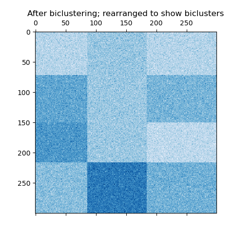
現在,我們根據 SpectralBiclustering 模型分配的行和列標簽按升序重新排列數據,并再次繪制。row_labels_ 的范圍從 0 到 3,而 column_labels_ 的范圍從 0 到 2,代表每行有 4 個簇,每列有 3 個簇。
# 首先重新排列行,然后是列。
reordered_rows = data[np.argsort(model.row_labels_)]
reordered_data = reordered_rows[:, np.argsort(model.column_labels_)]plt.matshow(reordered_data, cmap=plt.cm.Blues)
plt.title("二分聚類后;重新排列以顯示二分聚類")
plt.show()
最后一步,我們想展示模型分配的行和列標簽之間的關系。因此,我們使用 numpy.outer 創建一個網格,它將排序后的 row_labels_ 和 column_labels_ 相加 1,以確保標簽從 1 開始而不是 0,以便更好地可視化。
plt.matshow(np.outer(np.sort(model.row_labels_) + 1, np.sort(model.column_labels_) + 1), cmap=plt.cm.Blues)
plt.title("重新排列數據的方格結構")
plt.show()
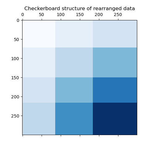
行和列標簽向量的外積顯示了方格結構的表示,其中不同的行和列標簽組合用不同的藍色陰影表示。
腳本的總運行時間:(0 分鐘 0.534 秒)
- 啟動 binder : https://mybinder.org/v2/gh/scikit-learn/scikit-learn/1.6.X?urlpath=lab/tree/notebooks/auto_examples/bicluster/plot_spectral_biclustering.ipynb
- 啟動 JupyterLite : https://scikit-learn.org/stable/lite/lab/index.html?path=auto_examples/bicluster/plot_spectral_biclustering.ipynb
- 下載 Jupyter notebook:`plot_spectral_biclustering.ipynb](https://scikit-learn.org/stable/_downloads//6b00e458f3e282f1cc421f077b2fcad1/plot_spectral_biclustering.ipynb>
- 下載 Python 源代碼:
plot_spectral_biclustering.py: https://scikit-learn.org/stable/_downloads//ac19db97f4bbd077ccffef2736ed5f3d/plot_spectral_biclustering.py - 下載 zip 文件:
plot_spectral_biclustering.zip: <https://scikit-learn.org/stable/_downloads//f66c3a9f3631c05c52d31172371922ab/plot_spectral_biclustering.zip`
Spectral Co-Clustering 算法演示
本例演示了如何使用 Spectral Co-Clustering 算法生成數據集并對其進行二分聚類。
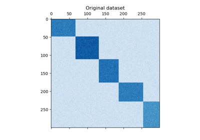
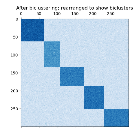
數據集使用 make_biclusters 函數生成,該函數創建一個包含小值的矩陣,并植入具有大值的大值二分塊。然后,行和列進行洗牌,并傳遞給 Spectral Co-Clustering 算法。通過重新排列洗牌后的矩陣以顯示連續的二分塊,展示了算法找到二分塊的高準確性。
一致性得分:1.000
# 作者:scikit-learn 開發者
# SPDX-License-Identifier: BSD-3-Clauseimport numpy as np
from matplotlib import pyplot as pltfrom sklearn.cluster import [SpectralCoclustering](https://scikit-learn.org/stable/modules/generated/sklearn.cluster.SpectralCoclustering.html#sklearn.cluster.SpectralCoclustering "sklearn.cluster.SpectralCoclustering")
from sklearn.datasets import [make_biclusters](https://scikit-learn.org/stable/modules/generated/sklearn.datasets.make_biclusters.html#sklearn.datasets.make_biclusters "sklearn.datasets.make_biclusters")
from sklearn.metrics import [consensus_score](https://scikit-learn.org/stable/modules/generated/sklearn.metrics.consensus_score.html#sklearn.metrics.consensus_score "sklearn.metrics.consensus_score")data, rows, columns = [make_biclusters](https://scikit-learn.org/stable/modules/generated/sklearn.datasets.make_biclusters.html#sklearn.datasets.make_biclusters "sklearn.datasets.make_biclusters")(shape=(300, 300), n_clusters=5, noise=5, shuffle=False, random_state=0
)[plt.matshow](https://matplotlib.org/stable/api/_as_gen/matplotlib.pyplot.matshow.html#matplotlib.pyplot.matshow "matplotlib.pyplot.matshow")(data, cmap=plt.cm.Blues)
[plt.title](https://matplotlib.org/stable/api/_as_gen/matplotlib.pyplot.title.html#matplotlib.pyplot.title "matplotlib.pyplot.title")("原始數據集")# 洗牌聚類
rng = [np.random.RandomState](https://numpy.org/doc/stable/reference/random/legacy.html#numpy.random.RandomState "numpy.random.RandomState")(0)
row_idx = rng.permutation(data.shape[0])
col_idx = rng.permutation(data.shape[1])
data = data[row_idx][:, col_idx][plt.matshow](https://matplotlib.org/stable/api/_as_gen/matplotlib.pyplot.matshow.html#matplotlib.pyplot.matshow "matplotlib.pyplot.matshow")(data, cmap=plt.cm.Blues)
[plt.title](https://matplotlib.org/stable/api/_as_gen/matplotlib.pyplot.title.html#matplotlib.pyplot.title "matplotlib.pyplot.title")("洗牌后的數據集")model = [SpectralCoclustering](https://scikit-learn.org/stable/modules/generated/sklearn.cluster.SpectralCoclustering.html#sklearn.cluster.SpectralCoclustering "sklearn.cluster.SpectralCoclustering")(n_clusters=5, random_state=0)
model.fit(data)
score = [consensus_score](https://scikit-learn.org/stable/modules/generated/sklearn.metrics.consensus_score.html#sklearn.metrics.consensus_score "sklearn.metrics.consensus_score")(model.biclusters_, (rows[:, row_idx], columns[:, col_idx]))print("一致性得分:{:.3f}".format(score))fit_data = data[[np.argsort](https://numpy.org/doc/stable/reference/generated/numpy.argsort.html#numpy.argsort "numpy.argsort")(model.row_labels_)]
fit_data = fit_data[:, [np.argsort](https://numpy.org/doc/stable/reference/generated/numpy.argsort.html#numpy.argsort "numpy.argsort")(model.column_labels_)][plt.matshow](https://matplotlib.org/stable/api/_as_gen/matplotlib.pyplot.matshow.html#matplotlib.pyplot.matshow "matplotlib.pyplot.matshow")(fit_data, cmap=plt.cm.Blues)
[plt.title](https://matplotlib.org/stable/api/_as_gen/matplotlib.pyplot.title.html#matplotlib.pyplot.title "matplotlib.pyplot.title")("二分聚類后;重新排列以顯示二分塊")[plt.show](https://matplotlib.org/stable/api/_as_gen/matplotlib.pyplot.show.html#matplotlib.pyplot.show "matplotlib.pyplot.show")()
腳本的總運行時間: (0 分鐘 0.347 秒)
- 啟動 binder : https://mybinder.org/v2/gh/scikit-learn/scikit-learn/1.6.X?urlpath=lab/tree/notebooks/auto_examples/bicluster/plot_spectral_coclustering.ipynb
- 啟動 JupyterLite : https://scikit-learn.org/stable/lite/lab/index.html?path=auto_examples/bicluster/plot_spectral_coclustering.ipynb
- 下載 Jupyter notebook:`plot_spectral_coclustering.ipynb](https://scikit-learn.org/stable/_downloads//ee8e74bb66ae2967f890e19f28090b37/plot_spectral_coclustering.ipynb>
- 下載 Python 源代碼:
plot_spectral_coclustering.py: https://scikit-learn.org/stable/_downloads//bc8849a7cb8ea7a8dc7237431b95a1cc/plot_spectral_coclustering.py - 下載 zip 文件:
plot_spectral_coclustering.zip: <https://scikit-learn.org/stable/_downloads//3019a99f3f124514f9a0650bcb33fa27/plot_spectral_coclustering.zip`
使用光譜協同聚類算法進行文檔的二分聚類
本例展示了如何使用光譜協同聚類算法對二十個新聞組數據集進行處理。由于“comp.os.ms-windows.misc”類別包含大量僅包含數據的帖子,因此該類別被排除。
TF-IDF 向量化后的帖子形成了一個詞頻矩陣,然后使用 Dhillon 的光譜協同聚類算法進行二分聚類。結果文檔-詞二分聚類表示了那些子文檔中更常用的一些子詞。
對于一些最好的二分聚類,打印出其最常見的文檔類別和十個最重要的詞。最好的二分聚類是由其歸一化切割確定的。最好的詞是通過比較其在二分聚類內外部的和來確定的。
為了比較,文檔還使用 MiniBatchKMeans 進行了聚類。從二分聚類中得到的文檔簇比 MiniBatchKMeans 找到的簇的 V-measure 更好。
向量化...
協同聚類...
完成耗時 1.20 秒。V-measure: 0.4415
MiniBatchKMeans...
完成耗時 2.28 秒。V-measure: 0.3015最佳二分聚類:
----------------
二分聚類 0 : 8 個文檔,6 個詞
類別   : 100% talk.politics.mideast
詞        : cosmo, angmar, alfalfa, alphalpha, proline, benson二分聚類 1 : 1948 個文檔,4325 個詞
類別   : 23% talk.politics.guns, 18% talk.politics.misc, 17% sci.med
詞        : gun, guns, geb, banks, gordon, clinton, pitt, cdt, surrender, veal二分聚類 2 : 1259 個文檔,3534 個詞
類別   : 27% soc.religion.christian, 25% talk.politics.mideast, 25% alt.atheism
詞        : god, jesus, christians, kent, sin, objective, belief, christ, faith, moral二分聚類 3 : 775 個文檔,1623 個詞
類別   : 30% comp.windows.x, 25% comp.sys.ibm.pc.hardware, 20% comp.graphics
詞        : scsi, nada, ide, vga, esdi, isa, kth, s3, vlb, bmug二分聚類 4 : 2180 個文檔,2802 個詞
類別   : 18% comp.sys.mac.hardware, 16% sci.electronics, 16% comp.sys.ibm.pc.hardware
詞        : voltage, shipping, circuit, receiver, processing, scope, mpce, analog, kolstad, umass
# Authors: The scikit-learn developers
# SPDX-License-Identifier: BSD-3-Clause
from collections import Counter
from time import timeimport numpy as npfrom sklearn.cluster import MiniBatchKMeans, SpectralCoclustering
from sklearn.datasets import fetch_20newsgroups
from sklearn.feature_extraction.text import TfidfVectorizer
from sklearn.metrics.cluster import v_measure_scoredef number_normalizer(tokens):"""將所有數字標記映射到占位符。對于許多應用,以數字開頭的標記不是直接有用的,但這樣的標記存在的事實可能很重要。通過應用這種形式的降維,某些方法可能表現得更好。"""return ("#NUMBER" if token[0].isdigit() else token for token in tokens)class NumberNormalizingVectorizer(TfidfVectorizer):def build_tokenizer(self):tokenize = super().build_tokenizer()return lambda doc: list(number_normalizer(tokenize(doc)))# 排除 'comp.os.ms-windows.misc'
categories = ["alt.atheism", "comp.graphics", "comp.sys.ibm.pc.hardware", "comp.sys.mac.hardware", "comp.windows.x", "misc.forsale", "rec.autos", "rec.motorcycles", "rec.sport.baseball", "rec.sport.hockey", "sci.crypt", "sci.electronics", "sci.med", "sci.space", "soc.religion.christian", "talk.politics.guns", "talk.politics.mideast", "talk.politics.misc", "talk.religion.misc", ]
newsgroups = fetch_20newsgroups(categories=categories)
y_true = newsgroups.targetvectorizer = NumberNormalizingVectorizer(stop_words="english", min_df=5)
cocluster = SpectralCoclustering(n_clusters=len(categories), svd_method="arpack", random_state=0
)
kmeans = MiniBatchKMeans(n_clusters=len(categories), batch_size=20000, random_state=0, n_init=3
)print("向量化...")
X = vectorizer.fit_transform(newsgroups.data)print("協同聚類...")
start_time = time()
cocluster.fit(X)
y_cocluster = cocluster.row_labels_
print(f"完成耗時 {time() - start_time:.2f}s. V-measure: {v_measure_score(y_cocluster, y_true):.4f}"
)print("MiniBatchKMeans...")
start_time = time()
y_kmeans = kmeans.fit_predict(X)
print(f"完成耗時 {time() - start_time:.2f}s. V-measure: {v_measure_score(y_kmeans, y_true):.4f}"
)feature_names = vectorizer.get_feature_names_out()
document_names = list(newsgroups.target_names[i] for i in newsgroups.target)def bicluster_ncut(i):rows, cols = cocluster.get_indices(i)if not (np.any(rows) and np.any(cols)):import sysreturn sys.float_info.maxrow_complement = np.nonzero(np.logical_not(cocluster.rows_[i]))[0]col_complement = np.nonzero(np.logical_not(cocluster.columns_[i]))[0]# 注意:以下與 X[rows[:, np.newaxis], cols].sum() 相同,但在 scipy <= 0.16 中更快weight = X[rows][:, cols].sum()cut = X[row_complement][:, cols].sum() + X[rows][:, col_complement].sum()return cut / weightbicluster_ncuts = list(bicluster_ncut(i) for i in range(len(newsgroups.target_names)))
best_idx = np.argsort(bicluster_ncuts)[:5]print()
print("最佳二分聚類:")
print("----------------")
for idx, cluster in enumerate(best_idx):n_rows, n_cols = cocluster.get_shape(cluster)cluster_docs, cluster_words = cocluster.get_indices(cluster)if not len(cluster_docs) or not len(cluster_words):continue# 類別counter = Counter(document_names[doc] for doc in cluster_docs)cat_string = ", ".join(f"{(c / n_rows * 100):.0f}% {name}" for name, c in counter.most_common(3))# 詞out_of_cluster_docs = cocluster.row_labels_ != clusterout_of_cluster_docs = np.where(out_of_cluster_docs)[0]word_col = X[:, cluster_words]word_scores = np.array(word_col[cluster_docs, :].sum(axis=0)- word_col[out_of_cluster_docs, :].sum(axis=0))word_scores = word_scores.ravel()important_words = list(feature_names[cluster_words[i]] for i in word_scores.argsort()[:-11:-1])print(f"二分聚類 {idx} : {n_rows} 個文檔,{n_cols} 個詞")print(f"類別   : {cat_string}")print(f"詞        : {', '.join(important_words)}\n")
腳本的總運行時間: (0 分鐘 15.176 秒)
- 啟動 binder : https://mybinder.org/v2/gh/scikit-learn/scikit-learn/1.6.X?urlpath=lab/tree/notebooks/auto_examples/bicluster/plot_bicluster_newsgroups.ipynb
- 啟動 JupyterLite : https://scikit-learn.org/stable/lite/lab/index.html?path=auto_examples/bicluster/plot_bicluster_newsgroups.ipynb
- 下載 Jupyter notebook: plot_bicluster_newsgroups.ipynb](https://scikit-learn.org/stable/_downloads//3f7191b01d0103d1886c959ed7687c4d/plot_bicluster_newsgroups.ipynb>
- 下載 Python 源代碼: plot_bicluster_newsgroups.py` : https://scikit-learn.org/stable/_downloads//e68419b513284db108081422c73a5667/plot_bicluster_newsgroups.py
- 下載 zip 文件: plot_bicluster_newsgroups.zip
: <https://scikit-learn.org/stable/_downloads//ccd24a43e08ccb154430edf7f927cfc7/plot_bicluster_newsgroups.zip


)


)


_常規的電源管理的基本概念和軟件架構)


)
