深度學習(魚書)day06–神經網絡的學習(后兩節)
一、梯度
像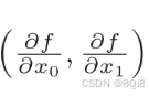
這樣的由全部變量的偏導數匯總而成的向量稱為梯度(gradient)。
梯度實現的代碼:
def numerical_gradient(f, x):h = 1e-4 # 0.0001grad = np.zeros_like(x) # 生成和x形狀相同的數組for idx in range(x.size):tmp_val = x[idx]# f(x+h)的計算x[idx] = tmp_val + hfxh1 = f(x)# f(x-h)的計算x[idx] = tmp_val - h fxh2 = f(x)grad[idx] = (fxh1 - fxh2) / (2*h)x[idx] = tmp_val # 還原值return grad
這里我們求點(3,4)、(0,2)、(3,0)處的梯度。
numerical_gradient(function_2, np.array([3.0, 4.0]))
# array([ 6., 8.])
numerical_gradient(function_2, np.array([0.0, 2.0]))
# array([ 0., 4.])
numerical_gradient(function_2, np.array([3.0, 0.0]))
# array([ 6., 0.])
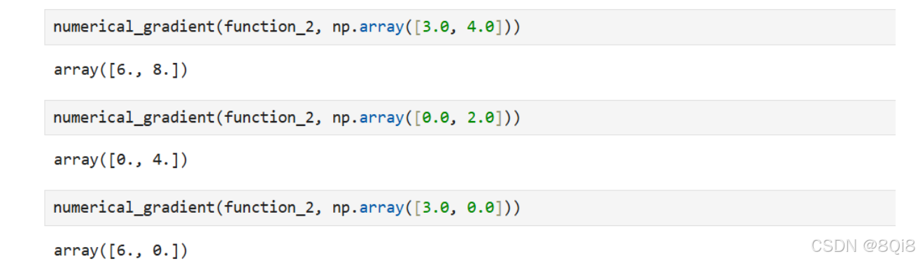
這里我們畫的是元素值為負梯度的向量,梯度指向函數f(x0,x1)的“最低處”(最小值),就像指南針一樣,所有的箭頭都指向同一點。其次,我們發現離“最低處”越遠,箭頭越大。
梯度會指向各點處的函數值降低的方向。更嚴格地講,梯度指示的方向是各點處的函數值減小最多的方向。在復雜的函數中,梯度指示的方向基本上都不是函數值最小處。
-
梯度法:通過不斷地沿梯度方向前進,逐漸減小函數值的過程就是梯度法(gradient method)
-
函數的極小值、最小值以及被稱為鞍點(saddle point)的地方,梯度為 0。雖然梯度法是要尋找梯度為 0的地方,但是那個地方不一定就是最小值(也有可能是極小值或者鞍點)。當函數很復雜且呈扁平狀時,學習可能會進入一個(幾乎)平坦的地區,陷入被稱為“學習高原”的無法前進的停滯期。
-
雖然梯度的方向并不一定指向最小值,但沿著它的方向能夠最大限度地減小函數的值。因此,在尋找函數的最小值(或者盡可能小的值)的位置的任務中,要以梯度的信息為線索,決定前進的方向。
-
尋找最小值的梯度法稱為梯度下降法(gradient descent method),尋找最大值的梯度法稱為梯度上升法(gradient ascent method)。 但是 通過反轉損失函數的符號, 求最小值的問題和求最大值的問題會變成相同的問題,因此“下降”還是“上升”的差異本質上并不重要。一般來說,神經網絡(深度學習)中,梯度法主要是指梯度下降法。
數學式子表示梯度法:
x0=x0?η?f?x0x1=x1?η?f?x1 x_0 = x_0 - \eta \frac{\partial f}{\partial x_0} \\ x_1 = x_1 - \eta \frac{\partial f}{\partial x_1} x0?=x0??η?x0??f?x1?=x1??η?x1??f?
η表示更新量,在神經網絡的學習中,稱為學習率(learning rate)。學習率決定在一次學習中,應該學習多少,以及在多大程度上更新參數。這表示更新一次的式子,這個步驟會反復執行,逐漸減小函數值。在神經網絡的學習中,一般會一邊改變學習率的值,一邊確認學習是否正確進行了。
def gradient_descent(f,init_x,lr=0.01,step_sum=100):x = init_xfor i in range(step_num):grad = numerical_gradient(f, x)x -= lr * gradreturn x參數f是要進行最優化的函數,init_x是初始值,lr是學習率learning rate,step_num是梯度法的重復次數。
-

init_x = np.array([-3.0, 4.0])
gradient_descent(function_2,init_x,lr=0.1,step_num=100)
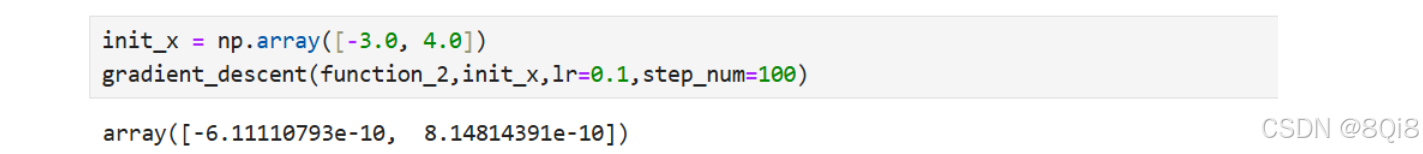
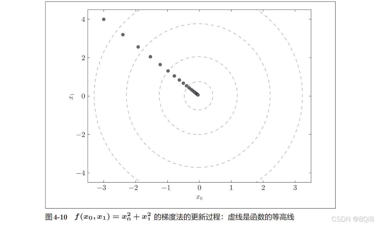
原點處是最低的地方,函數的取值一點點在向其靠近。
學習率過大或者過小都無法得到好的結果。我們來做個實驗驗證一下。
學習率過大的例子:lr=10.0
init_x = np.array([-3.0, 4.0])
gradient_descent(function_2, init_x=init_x, lr=10.0, step_num=100)
# array([ -2.58983747e+13, -1.29524862e+12])
學習率過小的例子:lr=1e-10
init_x = np.array([-3.0, 4.0])
gradient_descent(function_2, init_x=init_x, lr=1e-10, step_num=100)
# array([-2.99999994, 3.99999992])
實驗結果表明,學習率過大的話,會發散成一個很大的值;反過來,學習率過小的話,基本上沒怎么更新就結束了。
像學習率這樣的參數稱為超參數。這是一種和神經網絡的參數(權重和偏置)性質不同的參數。相對于神經網絡的權重參數是通過訓練數據和學習算法自動獲得的,學習率這樣的超參數則是人工設定的。一般來說,超參數需要嘗試多個值,以便找到一種可以使學習順利進行的設定。
-
神經網絡的梯度
神經網絡的學習也要求梯度,這里所說的梯度是指損失函數關于權重參數的梯度:
$$\boldsymbol{W} = \begin{pmatrix}
w_{11} & w_{12} & w_{13} \
w_{21} & w_{22} & w_{23}
\end{pmatrix}
\
\frac{\partial L}{\partial \boldsymbol{W}} = \begin{pmatrix}
\frac{\partial L}{\partial w_{11}} & \frac{\partial L}{\partial w_{12}} & \frac{\partial L}{\partial w_{13}} \
\frac{\partial L}{\partial w_{21}} & \frac{\partial L}{\partial w_{22}} & \frac{\partial L}{\partial w_{23}}
\end{pmatrix}
$$
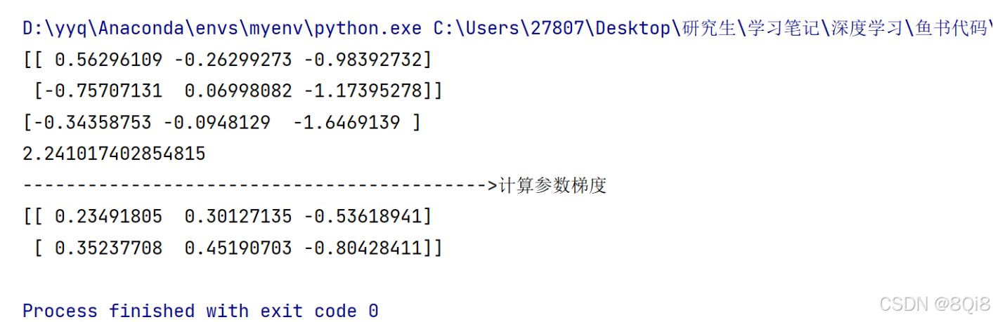
我們以一個簡單的神經網絡為例,來實現求梯度的代碼:import sys, os sys.path.append(os.pardir) # 為了導入父目錄中的文件而進行的設定 import numpy as np from common.functions import softmax, cross_entropy_error from common.gradient import numerical_gradientclass simpleNet:def __init__(self):self.W = np.random.randn(2, 3)def pridect(self,x):return np.dot(x,self.W)def loss(self,x,t):z = self.pridect(x)y = softmax(z)loss = cross_entropy_error(y, t)return lossnet = simpleNet() print(net.W)x = np.array([0.6, 0.9]) p = net.pridect(x) print(p) t = np.array([0, 0, 1]) loss = net.loss(x, t) print(loss) print("------------------------------------------->計算參數梯度") # def f(W): # return net.loss(x, t) f = lambda w: net.loss(x, t) dW = numerical_gradient(f, net.W) print(dW)
二、學習算法的實現
神經網絡的學習步驟:
前提
神經網絡存在合適的權重和偏置,調整權重和偏置以便擬合訓練數據的過程稱為“學習”。神經網絡的學習分成下面4個步驟。
步驟1(mini-batch)
從訓練數據中隨機選出一部分數據,這部分數據稱為mini-batch。我們的目標是減小mini-batch的損失函數的值。
步驟2(計算梯度)
為了減小mini-batch的損失函數的值,需要求出各個權重參數的梯度。梯度表示損失函數的值減小最多的方向。
步驟3(更新參數)
將權重參數沿梯度方向進行微小更新。
步驟4(重復)
重復步驟1、步驟2、步驟3。
這里使用的數據是隨機選擇的mini batch數據,所以又稱為隨機梯度下降法(stochastic gradient descent)。“隨機”指的是“隨機選擇的”的意思,隨機梯度下降法是“對隨機選擇的數據進行的梯度下降法”。深度學習的很多框架中,隨機梯度下降法一般由一個名為SGD的函數來實現。SGD來源于隨機梯度下降法的英文名稱的首字母。
我們來實現手寫數字識別的神經網絡。這里以2層神經網絡(隱藏層為1層的網絡)為對象,使用MNIST數據集進行學習。
-
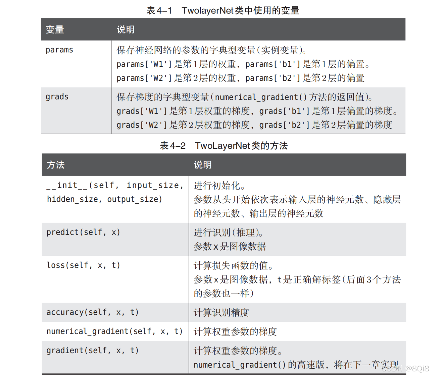
2層神經網絡的類
import sys, os
sys.path.append(os.pardir)
from common.functions import *
from common.gradient import numerical_gradientclass TwoLayerNet:def __init__(self, input_size, hidden_size, output_size, weight_init_std=0.01):self.params = {}self.params['W1'] = weight_init_std * np.random.randn(input_size, hidden_size)self.params['b1'] = np.zeros(hidden_size)self.params['W2'] = weight_init_std * np.random.randn(hidden_size, output_size)self.params['b2'] = np.zeros(output_size)def predict(self, x):W1, W2 = self.params['W1'],self.params['W2']b1, b2 = self.params['b1'],self.params['b2']a1 = np.dot(x, W1) + b1z1 = sigmoid(a1)a2 = np.dot(z1, W2) + b2y = softmax(a2)return ydef loss(self, x, t):y = self.predict(x)return cross_entropy_error(y, t)def accuracy(self, x, t):y = self.predict(x)y = np.argmax(y, axis=1)t = np.argmax(t, axis=1)accuracy = np.sum(y == t) / float(x.shape[0])return accuracydef numerical_gradient(self, x, t):loss_w = lambda w: self.loss(x, t)grads = {}grads['W1'] = numerical_gradient(loss_w, self.params['W1']) # 這里的numerical_gradient()是之前定義的求數值微分的函數grads['b1'] = numerical_gradient(loss_w, self.params['b1'])grads['W2'] = numerical_gradient(loss_w, self.params['W2'])grads['b2'] = numerical_gradient()def gradient(self, x, t):W1, W2 = self.params['W1'], self.params['W2']b1, b2 = self.params['b1'], self.params['b2']grads = {}batch_num = x.shape[0]a1 = np.dot(x, W1) + b1z1 = sigmoid(a1)a2 = np.dot(z1, W2) + b2y = softmax(a2)dy = (y - t) / batch_numgrads['W2'] = np.dot(z1.T, dy)grads['b2'] = np.sum(dy, axis=0)da1 = np.dot(dy, W2.T)dz1 = sigmoid_grad(a1) * da1grads['W1'] = np.dot(x.T, dz1)grads['b1'] = np.sum(dz1, axis=0)return grads
-
mini-batch的實現
所謂mini-batch學習,就是從訓練數據中隨機選擇一部分數據(稱為mini-batch),再以這些mini-batch為對象,使用梯度法更新參數的過程。下面,我們就以TwoLayerNet類為對象,使用MNIST數據集進行學習。
# coding: utf-8
import sys, os
sys.path.append(os.pardir)  # 為了導入父目錄的文件而進行的設定
import numpy as np
import matplotlib.pyplot as plt
from dataset.mnist import load_mnist
from two_layer_net import TwoLayerNet# 讀入數據
(x_train, t_train), (x_test, t_test) = load_mnist(normalize=True, one_hot_label=True)network = TwoLayerNet(input_size=784, hidden_size=50, output_size=10)iters_num = 10000  # 適當設定循環的次數
train_size = x_train.shape[0]
batch_size = 100
learning_rate = 0.1train_loss_list = []for i in range(iters_num):batch_mask = np.random.choice(train_size, batch_size)x_batch = x_train[batch_mask]t_batch = t_train[batch_mask]# 計算梯度#grad = network.numerical_gradient(x_batch, t_batch)grad = network.gradient(x_batch, t_batch)# 更新參數for key in ('W1', 'b1', 'W2', 'b2'):network.params[key] -= learning_rate * grad[key]loss = network.loss(x_batch, t_batch)train_loss_list.append(loss)
mini-batch的大小為100,需要每次從60000個訓練數據中隨機取出100個數據(圖像數據和正確解標簽數據)。然后,對這個包含100筆數據的mini-batch求梯度,使用隨機梯度下降法(SGD)更新參數。這里,梯度法的更新次數(循環的次數)為10000。每更新一次,都對訓練數據計算損失函數的值,并把該值添加到數組中。
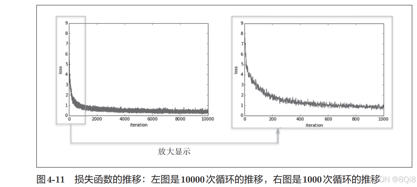
可以發現隨著學習的進行,損失函數的值在不斷減小。這是學習正常進行的信號,表示神經網絡的權重參數在逐漸擬合數據。
-
基于測試數據的評價
神經網絡的學習中,必須確認是否能夠正確識別訓練數據以外的其他數據,即確認是否會發生過擬合。過擬合是指,雖然訓練數據中的數字圖像能被正確辨別,但是不在訓練數據中的數字圖像卻無法被識別的現象。
- epoch是一個單位。一個 epoch表示學習中所有訓練數據均被使用過一次時的更新次數。比如,對于 10000筆訓練數據,用大小為 100筆數據的mini-batch進行學習時,重復隨機梯度下降法 100次,所有的訓練數據就都被“看過”了A。此時,100次就是一個 epoch。
完善代碼:
# coding: utf-8
import sys, os
sys.path.append(os.pardir)  # 為了導入父目錄的文件而進行的設定
import numpy as np
import matplotlib.pyplot as plt
from dataset.mnist import load_mnist
from two_layer_net import TwoLayerNet# 讀入數據
(x_train, t_train), (x_test, t_test) = load_mnist(normalize=True, one_hot_label=True)network = TwoLayerNet(input_size=784, hidden_size=50, output_size=10)iters_num = 10000  # 適當設定循環的次數
train_size = x_train.shape[0]
batch_size = 100
learning_rate = 0.1train_loss_list = []
train_acc_list = []
test_acc_list = []iter_per_epoch = max(train_size / batch_size, 1)for i in range(iters_num):batch_mask = np.random.choice(train_size, batch_size)x_batch = x_train[batch_mask]t_batch = t_train[batch_mask]# 計算梯度#grad = network.numerical_gradient(x_batch, t_batch)grad = network.gradient(x_batch, t_batch)# 更新參數for key in ('W1', 'b1', 'W2', 'b2'):network.params[key] -= learning_rate * grad[key]loss = network.loss(x_batch, t_batch)train_loss_list.append(loss)if i % iter_per_epoch == 0:train_acc = network.accuracy(x_train, t_train)test_acc = network.accuracy(x_test, t_test)train_acc_list.append(train_acc)test_acc_list.append(test_acc)print("train acc, test acc | " + str(train_acc) + ", " + str(test_acc))# 繪制圖形
markers = {'train': 'o', 'test': 's'}
x = np.arange(len(train_acc_list))
plt.plot(x, train_acc_list, label='train acc')
plt.plot(x, test_acc_list, label='test acc', linestyle='--')
plt.xlabel("epochs")
plt.ylabel("accuracy")
plt.ylim(0, 1.0)
plt.legend(loc='lower right')
plt.show()
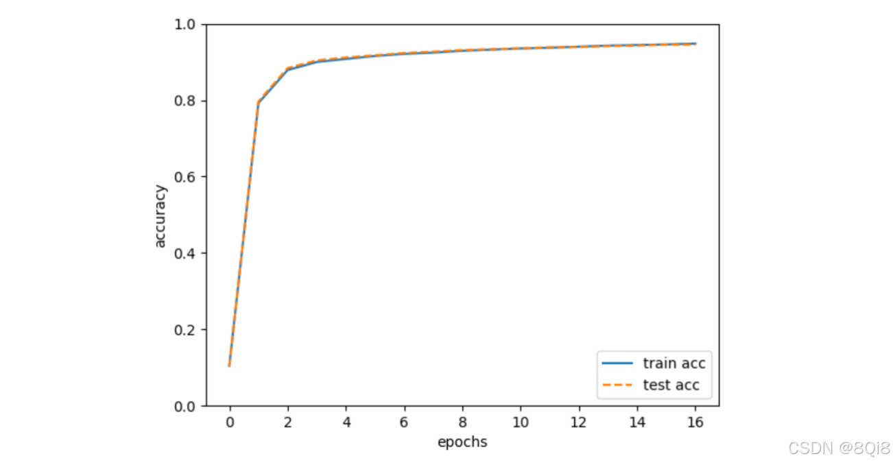
實線表示訓練數據的識別精度,虛線表示測試數據的識別精度。如圖所示,隨著epoch的前進(學習的進行),我們發現使用訓練數據和測試數據評價的識別精度都提高了,并且,這兩個識別精度基本上沒有差異(兩條線基本重疊在一起)。因此,可以說這次的學習中沒有發生過擬合的現象。
數據庫)


集成 openapi 插件)

:重新思考“組件”:狀態、視圖和邏輯的“最佳”分離實踐)

全面解析:從基礎到高級應用)
、組件通信)
——二叉樹應用:二叉樹選擇題)


的使用)
