JJCR一區 | Matlab實現GAF-PCNN-MATT、GASF-CNN、GADF-CNN的多特征輸入數據分類預測/故障診斷
目錄
- JJCR一區 | Matlab實現GAF-PCNN-MATT、GASF-CNN、GADF-CNN的多特征輸入數據分類預測/故障診斷
- 分類效果
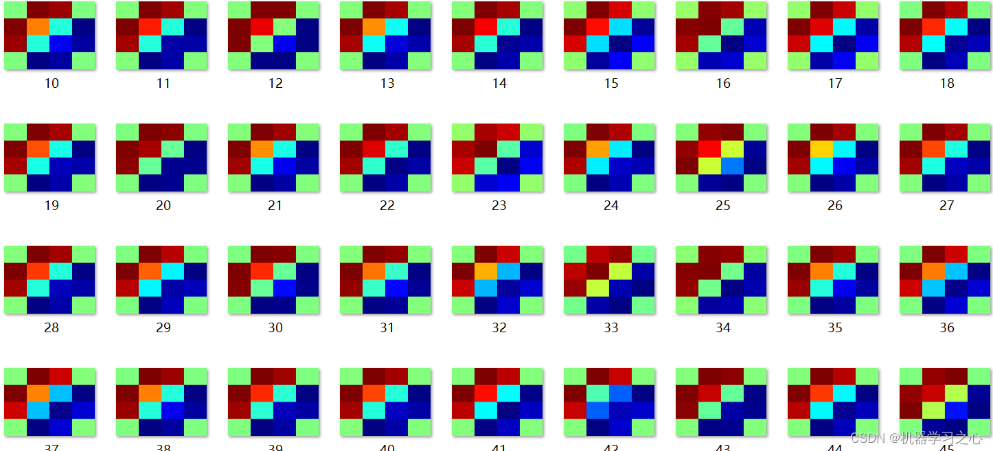
- 格拉姆矩陣圖
- GAF-PCNN-MATT
- GASF-CNN
- GADF-CNN
- 基本介紹
- 程序設計
- 參考資料
分類效果
格拉姆矩陣圖
GAF-PCNN-MATT


GASF-CNN


GADF-CNN


基本介紹
1.Matlab實現GAF-PCNN-MATT、GASF-CNN、GADF-CNN的多特征輸入數據分類預測/故障診斷,三個模型對比,運行環境matlab2023b;PCNN-MATT為并行卷積神經網絡融合多頭注意力機制。
2.先運行格拉姆矩陣變換進行數據轉換,然后運行分別GAF_PCNN-MATT.m,GADF_CNN.m,GASF_CNN.m完成多特征輸入數據分類預測/故障診斷;
GADF_CNN.m,是只用到了格拉姆矩陣的GADF矩陣,將GADF矩陣送入CNN進行故障診斷。
GASF_CNN-MATT.m,是只用到了格拉姆矩陣的GASF矩陣,將GASF矩陣送入CNN進行故障診斷。
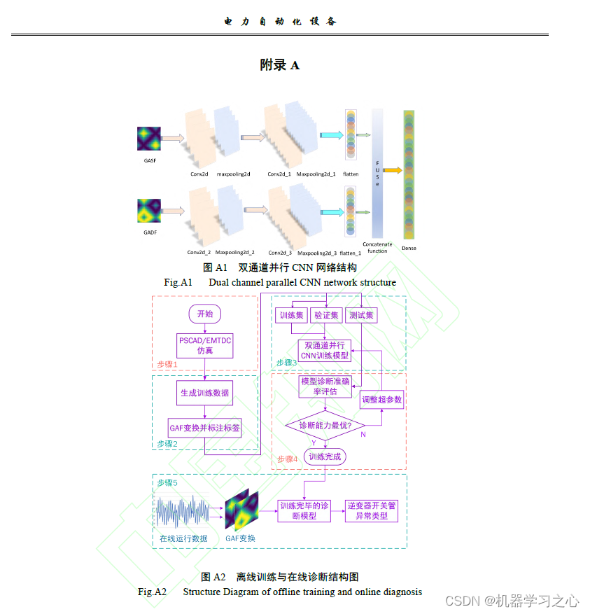
GAF_PCNN-MATT.m,是將GASF 圖與GADF 圖同時送入兩條并行CNN-MATT中,經過卷積-池化后,兩條CNN-MATT網絡各輸出一組一維向量;然后,將所輸出兩組一維向量進行拼接融合;通過全連接層后,最終將融合特征送入到Softmax 分類器中。
參考文獻

-
PCNN-MATT結構
-

-
CNN結構

程序設計
- 完整程序和數據獲取方式私信博主回復Matlab實現GAF-PCNN-MATT、GASF-CNN、GADF-CNN的多特征輸入數據分類預測/故障診斷。
fullyConnectedLayer(classnum,'Name','fc12')softmaxLayer('Name','softmax')classificationLayer('Name','classOutput')];lgraph = layerGraph(layers1);layers2 = [imageInputLayer([size(input2,1) size(input2,2)],'Name','vinput')  flattenLayer(Name='flatten2')bilstmLayer(15,'Outputmode','last','name','bilstm') dropoutLayer(0.1)        % Dropout層,以概率為0.2丟棄輸入reluLayer('Name','relu_2')selfAttentionLayer(2,2,"Name","mutilhead-attention")   %Attention機制fullyConnectedLayer(10,'Name','fc21')];
lgraph = addLayers(lgraph,layers2);
lgraph = connectLayers(lgraph,'fc21','add/in2');plot(lgraph)%% Set the hyper parameters for unet training
options = trainingOptions('adam', ...                 % 優化算法Adam'MaxEpochs', 1000, ...                            % 最大訓練次數'GradientThreshold', 1, ...                       % 梯度閾值'InitialLearnRate', 0.001, ...         % 初始學習率'LearnRateSchedule', 'piecewise', ...             % 學習率調整'LearnRateDropPeriod',700, ...                   % 訓練100次后開始調整學習率'LearnRateDropFactor',0.01, ...                    % 學習率調整因子'L2Regularization', 0.001, ...         % 正則化參數'ExecutionEnvironment', 'cpu',...                 % 訓練環境'Verbose', 1, ...                                 % 關閉優化過程'Plots', 'none');                    % 畫出曲線
%Code introduction
if nargin<2error('You have to supply all required input paremeters, which are ActualLabel, PredictedLabel')
end
if nargin < 3isPlot = true;
end%plotting the widest polygon
A1=1;
A2=1;
A3=1;
A4=1;
A5=1;
A6=1;a=[-A1 -A2/2 A3/2 A4 A5/2 -A6/2 -A1];
b=[0 -(A2*sqrt(3))/2 -(A3*sqrt(3))/2 0 (A5*sqrt(3))/2 (A6*sqrt(3))/2 0];if isPlotfigure   plot(a, b, '--bo','LineWidth',1.3)axis([-1.5 1.5 -1.5 1.5]);set(gca,'FontName','Times New Roman','FontSize',12);hold on%grid
end% Calculating the True positive (TP), False Negative (FN), False Positive...
% (FP),True Negative (TN), Classification Accuracy (CA), Sensitivity (SE), Specificity (SP),...
% Kappa (K) and F  measure (F_M) metrics
PositiveClass=max(ActualLabel);
NegativeClass=min(ActualLabel);
cp=classperf(ActualLabel,PredictedLabel,'Positive',PositiveClass,'Negative',NegativeClass);CM=cp.DiagnosticTable;TP=CM(1,1);FN=CM(2,1);FP=CM(1,2);TN=CM(2,2);CA=cp.CorrectRate;SE=cp.Sensitivity; %TP/(TP+FN)SP=cp.Specificity; %TN/(TN+FP)Pr=TP/(TP+FP);Re=TP/(TP+FN);F_M=2*Pr*Re/(Pr+Re);FPR=FP/(TN+FP);TPR=TP/(TP+FN);K=TP/(TP+FP+FN);[X1,Y1,T1,AUC] = perfcurve(ActualLabel,PredictedLabel,PositiveClass); %ActualLabel(1) means that the first class is assigned as positive class%plotting the calculated CA, SE, SP, AUC, K and F_M on polygon
x=[-CA -SE/2 SP/2 AUC K/2 -F_M/2 -CA];
y=[0 -(SE*sqrt(3))/2 -(SP*sqrt(3))/2 0 (K*sqrt(3))/2 (F_M*sqrt(3))/2 0];if isPlotplot(x, y, '-ko','LineWidth',1)set(gca,'FontName','Times New Roman','FontSize',12);
%     shadowFill(x,y,pi/4,80)fill(x, y,[0.8706 0.9216 0.9804])
end%calculating the PAM value
% Get the number of vertices
n = length(x);
% Initialize the area
p_area = 0;
% Apply the formula
for i = 1 : n-1p_area = p_area + (x(i) + x(i+1)) * (y(i) - y(i+1));
end
p_area = abs(p_area)/2;%Normalization of the polygon area to one.
PA=p_area/2.59807;if isPlot%Plotting the Polygonplot(0,0,'r+')plot([0 -A1],[0 0] ,'--ko')text(-A1-0.3, 0,'CA','FontWeight','bold','FontName','Times New Roman')plot([0 -A2/2],[0 -(A2*sqrt(3))/2] ,'--ko')text(-0.59,-1.05,'SE','FontWeight','bold','FontName','Times New Roman')plot([0 A3/2],[0 -(A3*sqrt(3))/2] ,'--ko')text(0.5, -1.05,'SP','FontWeight','bold','FontName','Times New Roman')plot([0 A4],[0 0] ,'--ko')text(A4+0.08, 0,'AUC','FontWeight','bold','FontName','Times New Roman')plot([0 A5/2],[0 (A5*sqrt(3))/2] ,'--ko')text(0.5, 1.05,'J','FontWeight','bold','FontName','Times New Roman')daspect([1 1 1])
end
Metrics.PA=PA;
Metrics.CA=CA;
Metrics.SE=SE;
Metrics.SP=SP;
Metrics.AUC=AUC;
Metrics.K=K;
Metrics.F_M=F_M;printVar(:,1)=categories;
printVar(:,2)={PA, CA, SE, SP, AUC, K, F_M};
disp('預測結果打印:')
for i=1:length(categories)fprintf('%23s: %.2f \n', printVar{i,1}, printVar{i,2})
end
參考資料
[1] https://blog.csdn.net/kjm13182345320/category_11799242.html?spm=1001.2014.3001.5482
[2] https://blog.csdn.net/kjm13182345320/article/details/124571691


與torch.no_grad())

)


通過社區投票將代幣遷移并更名為 CXT,以推動人工智能更深層次的創新)


,這樣既快速又高效,省去了“各種安裝+各種配置+各種遷移數據”帶來的麻煩和時間)

表達式(3)PAYLOAD EXPRESSIONS)
