提示：本篇博客是在閱讀了YOLO源碼中的mAP計算方法的代碼后加上官方解釋以及自己的debug調試理解每一步是怎么操作的。由于是大部分代碼進行了逐行解釋，所以篇幅過長。

---

前言

首先，在理解YOLO源碼中的mAP計算過程大部分參考了這篇文章：【目標檢測】評價指標：mAP概念及其代碼實現(yolo源碼/pycocotools)，這篇文章提到了mAP計算的一些基本知識，也提供了代碼，這里也是參考的這篇文章里的yolo源碼的mAP計算代碼（這篇文章是根據YOLO源碼中的整理過后的代碼）。想要源碼可以點鏈接進去或者本篇最后部分貼了源碼。

一、輸入格式處理

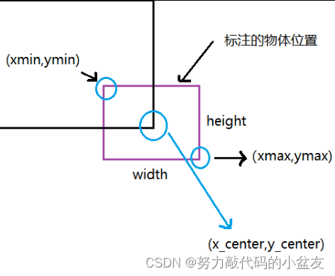
輸入的格式要求如下圖：

在進行mAP計算之前需要將YOLO模型預測文件的數據格式轉換為絕對位置，并且需要進行相應位置的轉換：
YOLO預測文件中：[class, $x_{center}$, $y_{center}$, width, height, conf] $\to$ [$x_{min}$, $y_{min}$, $x_{max}$, $y_{max}$, conf, class]
其中的$x_{center}$, $y_{center}$, width, height為相對位置，都是歸一化處理后的百分比位置，（$x_{min}$, $y_{min}$）,（ $x_{max}$, $y_{max}$）則是經過還原后在原圖上標注框的左上角和右下角在原圖中的坐標
真實結果同理進行轉換：我們在標注label的時候保存格式也是經過歸一化處理后的數據，在計算mAP的時候也需要還原到原圖的坐標上去。

1.1 轉換公式

此處的轉換原理和公式參考這篇文章所提到的標簽格式轉換：利用mAP計算yolo精確度，同時這篇文章也有格式轉換的代碼，大家可以參考，此處就不再貼格式轉換代碼，只簡述原理以及公式。
格式轉換的原理如下圖：

根據原理可以得到原始公式：
$$\begin{gathered} x_{center}=\frac{x_{min}+x_{max}}{2},y_{center}=\frac{y_{min}+y_{max}}{2}, \\ width=x_{max}?x_{min},height=y_{max}?y_{min} \end{gathered}$$
聯立上面四個公式可以得到：
$$\begin{gathered} x_{min}=x_{center}?\frac{width}{2},x_{max}=x_{center}+\frac{width}{2} \\ {y}_{min}=y_{center}?\frac{height}{2},y_{max}=y_{center}+\frac{height}{2} \end{gathered}$$
此時得到的（$x_{min}$, $y_{min}$）,（ $x_{max}$, $y_{max}$）是歸一化后的坐標，還需要進行原圖的還原：其中W、H為原圖的寬度和高度。ps：此處的W、H和width、height不是同一個東西，width和height是經過歸一化處理后的值，而W和H是原圖的寬高
$$\begin{gathered} x_{min}=x_{min}?W,x_{max}=x_{max}?W \\ {y}_{min}=y_{min}?H,y_{max}=y_{max}?H \end{gathered}$$

---

二、init：初始化

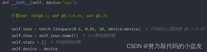
2.1 iouv

iouv就是從0.5到0.95分為10個值的數組

2.2 stats

stats是一個列表，包含4個numpy數組
stats[0] $\to$ shape：[$n_{pred}$，10] $\to$ 所有預測框載10個IOU閾值上是TP還是FP，其中$n_{pred}$表述所有預測框的總數量
stats[1] $\to$ shape：[$n_{pred}$] $\to$ 所有預測框的置信度
stats[2] $\to$ shape：[$n_{pred}$] $\to$ 所有預測框的預測類別
stats[3] $\to$ shape：[$n_{label}$] $\to$ 所有真實框（即label標簽的）的預測類別，其中$n_{label}$表述所有真實框的總數

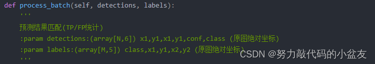
三、process_batch：實現預測結果和真實結果的匹配（TP/FP統計）

3.1 輸入參數的格式

在一部分已經闡述了格式的轉換，此處就不再進行贅述。
其中，N是預測框的總數，M是真實框的總數

3.2 代碼注釋（逐行）

# 每一個預測結果在不同IoU下的預測結果匹配
correct = np.zeros((detections.shape[0], self.niou)).astype(bool)

初始化correct（bool形式） $\to$ shape：[N, 10] $\to$ 在10個IOU閾值上每個預測框的TP、FP情況，True表示TP，False表示FP。
zeros即初始化全為0 $\to$ False

此處穿插python知識：使用shape可以快速讀取矩陣的形狀

# 二維矩陣
shape[0] # 讀取矩陣第一維度的長度 即數組的行數
shape[1] # 讀取矩陣第二維度的長度 即數組的列數# 圖像
image.shape[0] # 圖片的高
image.shape[1] # 圖片的寬
image.shape[2] # 圖片的通道數# 一般來說，在二維張量里，shape[-1]表示列數，
#注意，即使是一維行向量，shape[-1]表示行向量的元素總數，換言之也是列數：
shape[-1] # 表示最后一個維度

---

if detections is None:self.stats.append((correct, *torch.zeros((2, 0), device=self.device), labels[:, 0]))

注意一下：本地調試的時候，這里直接寫None會報錯
后面本人使用以下解決：當沒有產生預測文件的時候：使用tensor生成0行6列的向量。

 else: # 沒有預測框生成detections = torch.zeros((0, 6))

然后將上面從頭開始的兩句（correct的初始化以及判空的語句）修改為下面這個即可。

nl, npr = labels.shape[0], detections.shape[0]
correct = torch.zeros(npr, self.niou, dtype=torch.bool, device="cpu")if npr == 0:if nl:self.stats.append((correct, *torch.zeros((2, 0), device=self.device), labels[:, 0]))

---

else:# 計算標簽與所有預測結果之間的IoUiou = box_iou(labels[:, 1:], detections[:, :4])

iou $\to$ shape：[M,N]，以labels真實框為行，detections預測框為列 $\to$ 計算每個真實框與每個預測框之間的交并比IOU

---

   # 計算每一個預測結果可能對應的實際標簽correct_class = labels[:, 0:1] == detections[:, 5]

correct_class $\to$ shape：[M,N]，以labels真實框為行，detections預測框為列 $\to$ 保存每個真實框與每個預測框之間的類別是否相等，True即為類別一致，False即為類別不一致。
其中，labels[:, 0:1] == detections[:, 5]返回值為bool類型，True or False

例子：比如預測框預測的三個框的類別依次為2，0，1（括號里面表示類別，括號前面表示下標），真實框只有兩個框，并且類別依次為0，1。得到的correct_class矩陣如下所示

label\detection	0(2)	1(0)	2(1)
0(1)	F	F	T
1(2)	T	F	F

---

 for i in range(self.niou):  # 在不同IoU置信度下的預測結果匹配結果# 根據IoU置信度和類別對應得到預測結果與實際標簽的對應關系x = torch.where((iou >= self.iouv[i]) & correct_class)

外層的循環是指不同的IOU閾值下的計算
使用torch.where（此處采用的是后面所提的用法2：取Tensor中符合條件的坐標）獲得真實框和預測框之間的iou大于此時的IOU閾值并且類別一致的結果 $\to$ shape：[2, $N_{same}$] $\to$ $N_{same}$指的是一致的組總數量，第一行表示行坐標，第二行表示列坐標。

例子：假設前面獲得的iou和correct_class如下，此時的iou閾值為0.5，(0，2)(1，0)這兩組符合條件，成為返回的結果。故torch.where返回值為[ [0,1] [2,0] ]。（第一行表示真實框索引，第二行表示預測框索引）

iou：

label\detection	0(2)	1(0)	2(1)
0(1)	0.6	0.7	0.8
1(2)	0.9	0.2	0.1

correct_class：

label\detection	0(2)	1(0)	2(1)
0(1)	F	F	T
1(2)	T	F	F

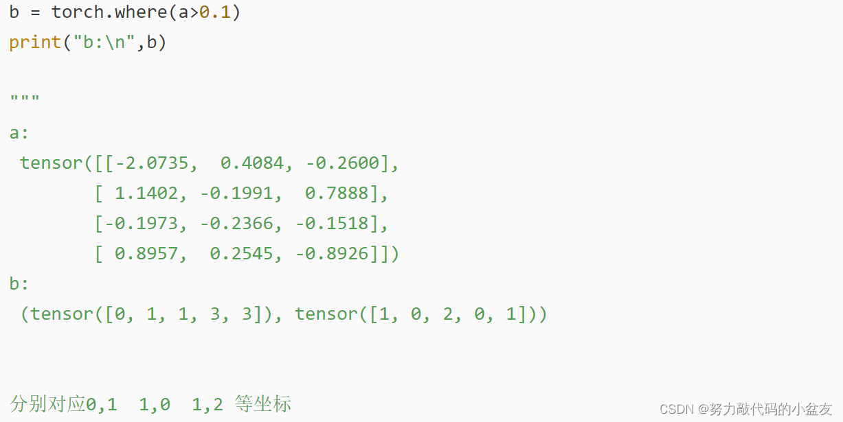
此處穿插python知識：torch.where用法
參考這篇文章：torch.where()的兩種用法

用法1：按照指定條件合并兩個同維度Tensor：
函數原型：torch.where(condition, x, y) $\to$ Tensor

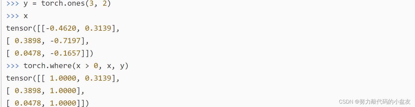
用法2：取Tensor中符合條件的坐標：
函數原型：torch.where(condition) $\to$ Tensor

---

# 若存在和實際標簽相匹配的預測結果
# x[0]:存在為True的索引(實際結果索引), x[1]當前所有True的索引(預測結果索引)
if x[0].shape[0]:  # [label, detect, iou]matches = torch.cat((torch.stack(x, 1), iou[x[0], x[1]][:, None]), 1).cpu().numpy()

通俗講，x[0]指的是x的第一行，即對應真實框的索引號。x[1]指的是x的第二行，即對應的預測框的索引號。如果x[0]存在，就進行一個[label, detect, iou]的拼接。

torch.stack(x, 1) $\to$ x在列上進行拼接，從[ [0,1] [2,0] ] $\to$ [ [0,2] [1,0] ]。相當于就是變回一組坐標的形式。
iou[x[0], x[1]][:, None] $\to$ 將iou矩陣中的對應于x中的索引的iou取出來，以[[0.8],[0.9]]的形式。
torch.cat((torch.stack(x, 1), iou[x[0], x[1]][:, None]), 1) $\to$ 將前面所得到的兩個東西在列上進行拼接 $\to$ 得到[ [0,2,0.8], [1,0,0.9] ] （形成[label, detect, iou]）

此處穿插python知識：torch.stack用法
沿一個新維度對輸入一系列張量進行連接，序列中所有張量應為相同形狀，stack 函數返回的結果會新增一個維度。

# dim = 0 : 在第0維進行連接，相當于在行上進行組合(輸入張量為一維，輸出張量為兩維)
a = torch.tensor([1, 2, 3])
b = torch.tensor([11, 22, 33])
c = torch.stack([a, b],dim=0)
#c => tensor([[ 1,  2,  3], [11, 22, 33]])# dim=1:在第1維進行連接，相當于在對應行上面對列元素進行組合(輸入張量為一維，輸出張量為兩維)
a = torch.tensor([1, 2, 3])
b = torch.tensor([11, 22, 33])
c = torch.stack([a, b],dim=1)
#c => tensor([[ 1, 11], [ 2, 22], [ 3, 33]])

此處穿插python知識：torch.cat用法
用于在指定的維度上拼接張量。這個函數接收一個張量列表，并在指定的維度上將它們連接起來。它通常用于連接兩個或多個張量，以創建一個更大的張量。

tensor1 = torch.tensor([[1, 2], [3, 4]])
tensor2 = torch.tensor([[5, 6], [7, 8]])
# 在第0維（行）上連接這兩個張量
result = torch.cat((tensor1, tensor2), dim=0)
# result => tensor([[1, 2], [3, 4], [5, 6], [7, 8]])
# 新的張量，行數=tensor1和tensor2 的行數之和，列數與 tensor1 和 tensor2 的列數相同。

---

   if x[0].shape[0] > 1:  # 存在多個與目標對應的預測結果# 根據IoU從高到低排序 [實際結果索引,預測結果索引,結果IoU]matches = matches[matches[:, 2].argsort()[::-1]] 

matches[:, 2].argsort()[::-1] $\to$ -1指的是逆序排序，即從IOU高到低排序，2是指matches[2]即iou值，整體返回的是逆序排位后的索引，如[1,0] （因為0.9>0.8，所以第二行應該和第一行交換位置，所以得到的排序后的索引為[1,0]）

再使用matches = matches[排序后的索引] 進行替換重置。

---

 # 每一個預測結果保留一個和實際結果的對應
matches = matches[np.unique(matches[:, 1], return_index=True)[1]] 
# 每一個實際結果和一個預測結果對應
matches = matches[np.unique(matches[:, 0], return_index=True)[1]]

np.unique(matches[:, 0], return_index=True)[0] => 去除重復后的值 [1] => 去除重復后的每個值對應的索引 [2] => dtype
然后matches再根據獲得去除重復后的索引進行排列。
ps：因為前面已經按照IOU從高到低進行排序了，故當去除的時候自動保留最高的IOU的那一組

此處穿插python知識：numpy.unique用法
此處參考這篇文章：【Python】np.unique() 介紹與使用
去除其中重復的元素 ，并按元素由小到大返回一個新的無元素重復的元組或者列表。

# 格式：numpy.unique(arr, return_index, return_inverse, return_counts)
# arr：輸入數組，如果不是一維數組則會展開
# return_index：如果為 true，返回新列表元素在舊列表中的位置（下標），并以列表形式存儲。
# return_inverse：如果為true，返回舊列表元素在新列表中的位置（下標），并以列表形式存儲。
# return_counts：如果為 true，返回去重數組中的元素在原數組中的出現次數。
A = [1, 2, 2, 5, 3, 4, 3]
a = np.unique(A) # [1 2 3 4 5]
a, indices = np.unique(A, return_index=True)# 返回新列表元素在舊列表中的位置（下標）
# a => [1 2 3 4 5] indices => [0 1 4 5 3]
a, indices = np.unique(A, return_inverse=True)# 舊列表的元素在新列表的位置
# a => [1 2 3 4 5] indices => [0 1 1 4 2 3 2]
a, indices = np.unique(A, return_counts=True)# 每個元素在舊列表里各自出現了幾次
# a => [1 2 3 4 5] indices => [1 2 2 1 1]

---

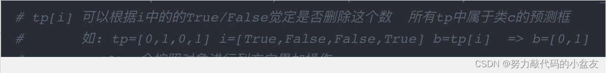
 # 表明當前預測結果在當前IoU下實現了目標的預測correct[matches[:, 1].astype(int), i] = True  

matches[:, 1].astype(int) $\to$ 將matches的1列（第二列，即預測框的索引）作為int類型
matches表明經過篩選后留下的預測框的索引，然后在correct矩陣中將其置為True，即表明在該閾值（i）下，此預測框為正確的預測（TP）。

---

   # 預測結果在不同IoU是否預測正確, 預測置信度, 預測類別, 實際類別self.stats.append((correct, detections[:, 4], detections[:, 5], labels[:, 0]))

當所有iou閾值循環完成后，stats添加篩選過后的四個Numpy數組：correct、conf、class、label_class。

---

一個小總結：

數組名	shape	意義
correct	[$N_{pred}$, 10]	$N_{pred}$表示所有預測框的數量，表示所有預測框在該IOU閾值下為TP還是FP
correct_class	[$N_{label}$, $N_{pred}$]	表明每組真實框與預測框之間的類別是否一致
x	[2,X]	經過類別和閾值篩選后剩下的X組數據的索引號，第一行表示行坐標，第二行表示列坐標
matches	[Y,3]	去除重復后剩下的Y組數據，[label, detection, iou]形式，表明預測框和真實框匹配的框的數據
stats	每一維都有四個數組	分別為correct、conf、class、label_class

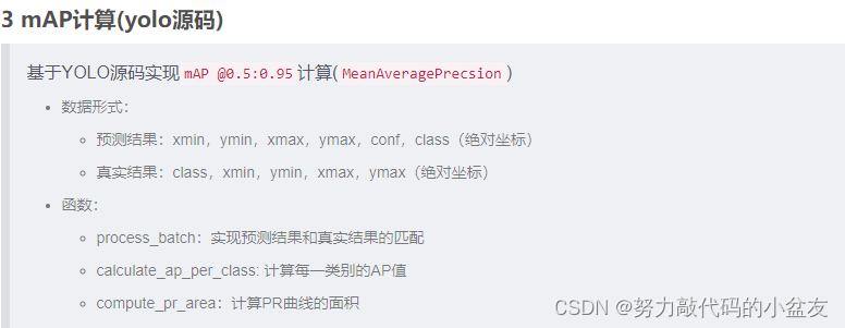
四、calculate_ap_per_class: 計算每一類別的AP值

4.1 代碼注釋（逐行）

stats = [torch.cat(x, 0).cpu().numpy() for x in zip(*self.stats)]  # to numpy
# tp:所有預測結果在不同IoU下的預測結果 [n, 10]
# conf: 所有預測結果的置信度
# pred_cls: 所有預測結果得到的類別
# target_cls: 所有圖片上的實際類別
tp, conf, pred_cls, target_cls = stats[0], stats[1], stats[2], stats[3]
# 根據類別置信度從大到小排序
i = np.argsort(-conf)  # 根據置信度從大到小排序
tp, conf, pred_cls = tp[i], conf[i], pred_cls[i]

第一行代碼是將所有圖片的四個數組進行匯總，在YOLO源碼中，未拼接前 $\to$ stats[0] 指第一張圖的四個數組，拼接后 $\to$ stats[0]指所有圖片的所有預測框的TP/FP情況。

然后再根據置信度逆序排序，即按照置信度從高到低進行排序。

---

# 得到所有類別及其對應數量(目標類別數)
unique_classes, nt = np.unique(target_cls, return_counts=True)
nc = unique_classes.shape[0]  # number of classes
# ap: 每一個類別在不同IoU置信度下的AP，shape[nc類別數, 10], 
# p:每一個類別的P曲線(不同類別置信度), r:每一個類別的R(不同類別置信度)
ap, p, r = np.zeros((nc, tp.shape[1])), np.zeros((nc, 1000)), np.zeros((nc, 1000))

np.unique用法見前面，此處不再贅述。

---

for ci, c in enumerate(unique_classes):  # 對每一個類別進行P,R計算，ci為c的index，c為值i = pred_cls == cn_l = nt[ci]  # number of labels 該類別的實際數量(正樣本數量)n_p = i.sum()  # number of predictions 預測結果數量if n_p == 0 or n_l == 0:continue

i = pred_cls == c返回的是bool類型的一維數組。
nt指的是每個類別真實框的總數量，一維數組。

---

# cumsum：軸向的累加和, 計算當前類別在不同的類別置信度下的P,R
fpc = (1 - tp[i]).cumsum(0)  # FP累加和(預測為負樣本且實際為負樣本)
tpc = tp[i].cumsum(0)  # TP累加和(預測為正樣本且實際為正樣本)
# 召回率計算(不同的類別置信度下)
recall = tpc / (n_l + eps)
# 精確率計算(不同的類別置信度下)
precision = tpc / (tpc + fpc)

TP和FP的計算方式開頭所提到的參考文章有非常清楚的解釋，此處不再贅述。
此處說一下tp[i]的用法見下圖，前面獲得了i這個數組，記錄了在tp數組中哪些預測框是當前類別的預測框。
tp[i]會保留對應i為True的數據。

cumsum(）的用法見圖

import numpy as np
a = np.asarray([[1, 2, 3],[4, 5, 6],[7, 8, 9]])
b = a.cumsum(axis=0) # 按行累加
# b=>[[1 2 3] [5 7 9] [12 15 18]]
c = a.cumsum(axis=1) # 按列累加
# c=>[[1 3 6] [4 9 15] [7 15 24]]

---

            # 計算不同類別置信度下的AP(根據P-R曲線計算)for j in range(tp.shape[1]):ap[ci, j], mpre, mrec = self.compute_ap(recall[:, j], precision[:, j])# 所有類別的ap值 @0.5:0.95return ap

最后得到recall和precision值后就是計算ap值。

五、compute_ap：計算PR曲線的面積

此處就是計算每一組PR值形成的曲線的面積，代碼本來的注解就很清晰明了，此處就不逐行解釋了。
此處貼一個插值積分求面積的博客，里面比較詳細介紹了插值積分：numpy.interp()用法

六、源碼

class MeanAveragePrecison:def __init__(self, device="cpu"):'''計算mAP: mAP@0.5; mAP @0.5:0.95; mAP @0.75'''self.iouv = torch.linspace(0.5, 0.95, 10, device=device)  # 不同的IoU置信度 @0.5:0.95self.niou = self.iouv.numel()  # IoU置信度數量self.stats = []  # 存儲預測結果self.device = devicedef process_batch(self, detections, labels):'''預測結果匹配(TP/FP統計):param detections:(array[N,6]) x1,y1,x1,y1,conf,class (原圖絕對坐標):param labels:(array[M,5]) class,x1,y1,x2,y2 (原圖絕對坐標)'''# 每一個預測結果在不同IoU下的預測結果匹配correct = np.zeros((detections.shape[0], self.niou)).astype(bool)if detections is None:self.stats.append((correct, *torch.zeros((2, 0), device=self.device), labels[:, 0]))else:# 計算標簽與所有預測結果之間的IoUiou = box_iou(labels[:, 1:], detections[:, :4])# 計算每一個預測結果可能對應的實際標簽correct_class = labels[:, 0:1] == detections[:, 5]for i in range(self.niou):  # 在不同IoU置信度下的預測結果匹配結果# 根據IoU置信度和類別對應得到預測結果與實際標簽的對應關系x = torch.where((iou >= self.iouv[i]) & correct_class)# 若存在和實際標簽相匹配的預測結果if x[0].shape[0]:  # x[0]:存在為True的索引(實際結果索引), x[1]當前所有True的索引(預測結果索引)# [label, detect, iou]matches = torch.cat((torch.stack(x, 1), iou[x[0], x[1]][:, None]), 1).cpu().numpy()if x[0].shape[0] > 1:  # 存在多個與目標對應的預測結果matches = matches[matches[:, 2].argsort()[::-1]]  # 根據IoU從高到低排序 [實際結果索引,預測結果索引,結果IoU]matches = matches[np.unique(matches[:, 1], return_index=True)[1]]  # 每一個預測結果保留一個和實際結果的對應matches = matches[np.unique(matches[:, 0], return_index=True)[1]]  # 每一個實際結果和一個預測結果對應correct[matches[:, 1].astype(int), i] = True  # 表面當前預測結果在當前IoU下實現了目標的預測# 預測結果在不同IoU是否預測正確, 預測置信度, 預測類別, 實際類別self.stats.append((correct, detections[:, 4], detections[:, 5], labels[:, 0]))def calculate_ap_per_class(self, save_dir='.', names=(), eps=1e-16):stats = [torch.cat(x, 0).cpu().numpy() for x in zip(*self.stats)]  # to numpy# tp:所有預測結果在不同IoU下的預測結果 [n, 10]# conf: 所有預測結果的置信度# pred_cls: 所有預測結果得到的類別# target_cls: 所有圖片上的實際類別tp, conf, pred_cls, target_cls = stats[0], stats[1], stats[2], stats[3]# 根據類別置信度從大到小排序i = np.argsort(-conf)  # 根據置信度從大到小排序tp, conf, pred_cls = tp[i], conf[i], pred_cls[i]# 得到所有類別及其對應數量(目標類別數)unique_classes, nt = np.unique(target_cls, return_counts=True)nc = unique_classes.shape[0]  # number of classes# ap: 每一個類別在不同IoU置信度下的AP, p:每一個類別的P曲線(不同類別置信度), r:每一個類別的R(不同類別置信度)ap, p, r = np.zeros((nc, tp.shape[1])), np.zeros((nc, 1000)), np.zeros((nc, 1000))for ci, c in enumerate(unique_classes):  # 對每一個類別進行P,R計算i = pred_cls == cn_l = nt[ci]  # number of labels 該類別的實際數量(正樣本數量)n_p = i.sum()  # number of predictions 預測結果數量if n_p == 0 or n_l == 0:continue# cumsum：軸向的累加和, 計算當前類別在不同的類別置信度下的P,Rfpc = (1 - tp[i]).cumsum(0)  # FP累加和(預測為負樣本且實際為負樣本)tpc = tp[i].cumsum(0)  # TP累加和(預測為正樣本且實際為正樣本)# 召回率計算(不同的類別置信度下)recall = tpc / (n_l + eps)# 精確率計算(不同的類別置信度下)precision = tpc / (tpc + fpc)# 計算不同類別置信度下的AP(根據P-R曲線計算)for j in range(tp.shape[1]):ap[ci, j], mpre, mrec = self.compute_ap(recall[:, j], precision[:, j])# 所有類別的ap值 @0.5:0.95return apdef compute_ap(self, recall, precision):# 增加初始值(P=1.0 R=0.0) 和 末尾值(P=0.0, R=1.0)mrec = np.concatenate(([0.0], recall, [1.0]))mpre = np.concatenate(([1.0], precision, [0.0]))# Compute the precision envelope np.maximun.accumulate# (返回一個數組,該數組中每個元素都是該位置及之前的元素的最大值)mpre = np.flip(np.maximum.accumulate(np.flip(mpre)))# 計算P-R曲線面積method = 'interp'  # methods: 'continuous', 'interp'if method == 'interp':  # 插值積分求面積x = np.linspace(0, 1, 101)  # 101-point interp (COCO))# 積分(求曲線面積)ap = np.trapz(np.interp(x, mrec, mpre), x)elif method == 'continuous':  # 不插值直接求矩陣面積i = np.where(mrec[1:] != mrec[:-1])[0]  # points where x axis (recall) changesap = np.sum((mrec[i + 1] - mrec[i]) * mpre[i + 1])  # area under curvereturn ap, mpre, mrec

---

結束語

淺淺記錄這幾天閱讀YOLO源碼中的mAP計算過程，自身python基礎不太ok，也算一邊查閱python語法知識一邊debug看懂每一步中數值的變化。可能以上自身的理解存在一點偏差，如果存在問題歡迎大家在評論區指出~