機器學習【五】decision

?決策樹是一種通過樹形結構進行數據分類或回歸的直觀算法，其核心是通過層級決策路徑模擬規則推理。主要算法包括：ID3算法基于信息熵和信息增益選擇劃分屬性；C4.5算法改進ID3，引入增益率和剪枝技術解決多值特征偏差；CART算法采用二叉樹結構，支持分類（基尼系數）與回歸（方差）任務。信用卡欺詐檢測案例實踐展示了全流程應用：通過SMOTE處理樣本不平衡，轉換時間特征及標準化數值完成數據預處理；利用網格搜索優化模型參數，可視化特征重要性與樹結構；設置動態閾值平衡誤報與漏報率，最終部署為實時檢測系統并定期更新模型。該案例驗證了決策樹在復雜業務場景中的解釋性與工程落地價值。

1 案例導學

想象你玩“20個問題”猜動物游戲：

問1：是哺乳動物嗎？→ 是

問2：有尾巴嗎？→ 是

問3：生活在水中嗎？→ 否

...

最后得出??答案是狗?🐕?

決策樹就是一套自動生成這種“問題流程”的算法，專治選擇困難癥！

2 決策樹

決策樹（Decision Tree），它是一種以樹形數據結構來展示決策規則和分類結果的模型，作為一種歸納學習算法，其重點是將看似無序、雜亂的已知數據，通過某種技術手段將它們轉化成可以預測未知數據的樹狀模型，每一條從根結點（對最終分類結果貢獻最大的屬性）到葉子結點（最終分類結果）的路徑都代表一條決策的規則。

當構建好決策樹后，那么分類和預測的任務就很簡單了，只需要走一遍就可以了，那么難點就在于如何構造出一棵樹。

構建流程

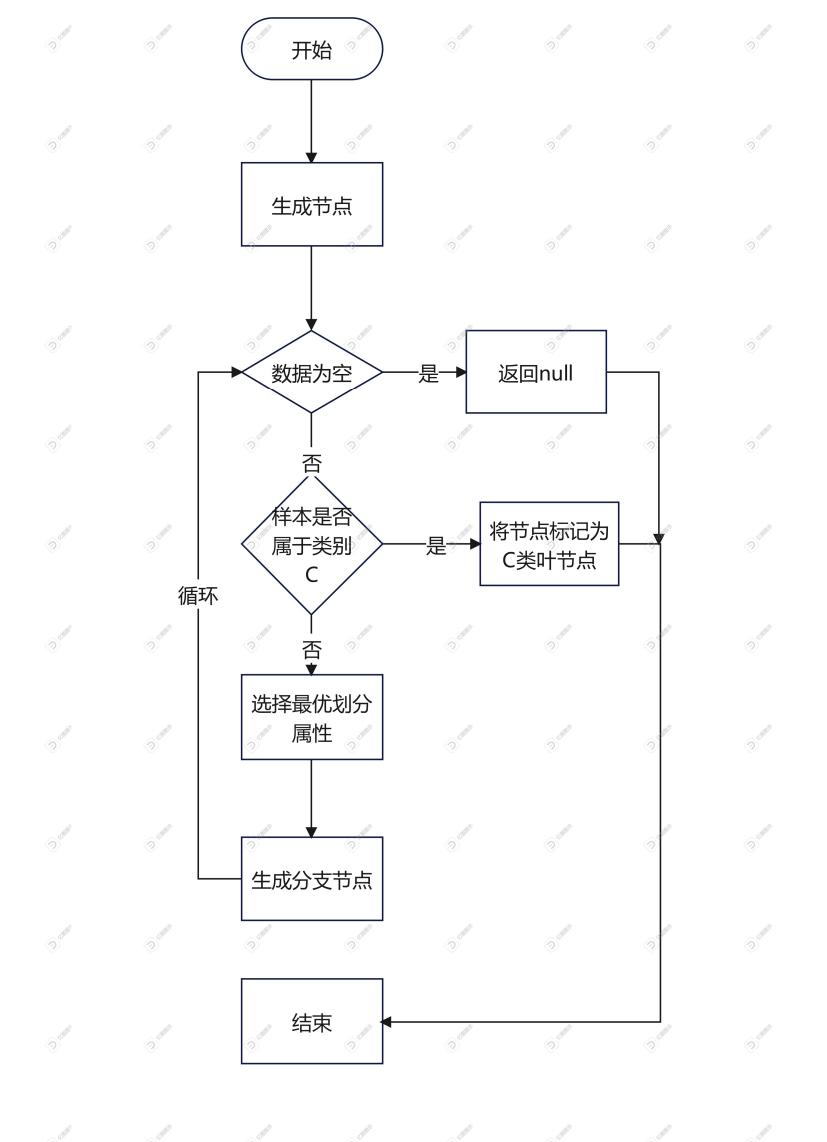
首先從開始位置，將所有數據劃分到一個節點，即根節點。
然后經歷橙色的兩個步驟，橙色的表示判斷條件：
若數據為空集，跳出循環。如果該節點是根節點，返回null；如果該節點是中間節點，將該節點標記為訓練數據中類別最多的類
若樣本都屬于同一類，跳出循環，節點標記為該類別；
如果經過橙色標記的判斷條件都沒有跳出循環，則考慮對該節點進行劃分。既然是算法，則不能隨意的進行劃分，要講究效率和精度，選擇當前條件下的最優屬性劃分（什么是最優屬性，這是決策樹的重點，后面會詳細解釋）
經歷上步驟劃分后，生成新的節點，然后循環判斷條件，不斷生成新的分支節點，直到所有節點都跳出循環。
結束。這樣便會生成一棵決策樹。

在執行決策樹生成的過程中，我們發現尋找最優劃分屬性是決策樹過程中的重點。那么如何在眾多的屬性中選擇最優的呢？下面我們學習三種算法。

3 ID3算法

ID3算法最早是由羅斯昆于1975提出的一種決策樹構建算法，算法的核心是“信息熵”。該算法是以信息論為基礎，以信息增益為衡量標準，從而實現對數據的歸納分類。而實際的算法流程是計算每個屬性的信息增益，并選取具有最高增益的屬性作為給定的測試屬性。

3.1 信息熵?

熵就是表示隨機變量不確定性的度量，物體內部的混亂程度。熵越大，系統越混亂。

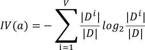
信息熵公式如下：

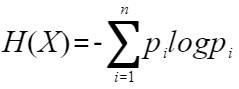
??X：?? 代表一個??離散隨機變量??，它有?n個可能的結果（或狀態）。例如：拋硬幣的結果（正、反），擲骰子的點數（1到6），明天天氣的類型（晴、雨、陰等），一個英文文本中的字母。
??p?：?? 代表隨機變量?X取第?i個可能結果發生的??概率??。例如，拋一枚公平硬幣，p(正面) = p(反面) = 0.5。擲一個公平骰子，p(點數為k) = 1/6。
??∑ (i=1 到 n)：?? 表示對所有可能的結果（從1到n）進行求和。
??log：?? 通常取??以2為底的對數 (log?)??。單位是??比特 (bit)??。有時也取自然對數 (ln)，單位是??納特 (nat)??。
??p? log p?：?? 這一項衡量了??單個結果 i 所貢獻的“驚奇度”或“信息量”??。注意，因為概率?p?在0到1之間，所以?log p?是負數（或零）。因此，我們加了一個負號?-。
??- p? log p?：?? 負號使這個量變成了??非負數??。p? log p?本身是個負值（因為概率小于等于1，其對數小于等于0），加上負號后就變成了正值。??-p? log p?可以理解為結果?i發生所能提供的期望信息量（基于其概率）。??
??H(X)：?? 對所有可能結果的?-p? log p?求和，得到的就是 ??X 的熵?H(X)。它代表了描述隨機變量?X（平均意義上）所需要的最小信息量（以比特或納特為單位），或者更根本地說，是?X本身的平均不確定性的度量。?

信息熵就是“萬物皆有其不確定性的數學度量”。它告訴我們，要描述一個不確定的東西，平均最少要多少信息。這個數字越大，那件事情就越“難猜”，越“出乎意料”。從扔硬幣到宇宙的復雜度，信息熵為我們理解隨機性和信息本身提供了一個強有力的量化工具。?

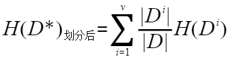
我們按照某一個屬性對數據進行劃分以后，得到第二個信息熵。

了解了信息熵以后，我們接下來認識一下信息增益。?

3.2 信息增益

信息增益：表示特征X使得類Y的不確定性減少的程度，分類后的專一性，希望分類后的結果是同類在一起。

其實就是劃分前的信息熵減去劃分后的信息熵。其中a代表的此次劃分中所使用的屬性。決策樹使用信息增益準則來選擇最優劃分屬性的話，在劃分前會針對每個屬性都計算信息增益，選擇能使得信息增益最大的屬性作為最優劃分屬性。

3.3 代碼實現

以“是否適合打網球”為例子簡單實現一下使用ID3的決策樹

# 使用ID3算法
import numpy as np
import math
from collections import Counterclass Node:"""決策樹節點類"""def __init__(self, feature=None, value=None, results=None, children=None):self.feature = feature  # 分割特征的索引self.value = value      # 特征值（用于判斷分支）self.results = results  # 葉節點的分類結果self.children = children # 子節點字典{特征值: 節點}def entropy(data):"""計算數據集的信息熵"""labels = [row[-1] for row in data]label_counts = Counter(labels)probs = [count / len(labels) for count in label_counts.values()]return -sum(p * math.log2(p) for p in probs)def split_data(data, feature_index, value):"""按指定特征分割數據集"""return [row for row in data if row[feature_index] == value]def information_gain(data, feature_index):"""計算特征的信息增益"""base_entropy = entropy(data)feature_values = {row[feature_index] for row in data}new_entropy = 0.0for value in feature_values:subset = split_data(data, feature_index, value)prob = len(subset) / len(data)new_entropy += prob * entropy(subset)return base_entropy - new_entropydef find_best_feature(data):"""尋找信息增益最大的特征"""best_gain = 0.0best_feature = -1# 最后1列是標簽，所以特征索引是0到len-2for feature_index in range(len(data[0]) - 1):gain = information_gain(data, feature_index)if gain > best_gain:best_gain = gainbest_feature = feature_indexreturn best_featuredef build_tree(data, feature_names):"""遞歸構建決策樹"""# 如果所有樣本屬于同一類別，返回葉節點labels = [row[-1] for row in data]if len(set(labels)) == 1:return Node(results=labels[0])# 選擇最佳分割特征best_feature_idx = find_best_feature(data)if best_feature_idx == -1:  # 如果沒有特征可選majority_label = Counter(labels).most_common(1)[0][0]return Node(results=majority_label)# 遞歸構建子樹feature_name = feature_names[best_feature_idx]unique_vals = {row[best_feature_idx] for row in data}children = {}for value in unique_vals:subset = split_data(data, best_feature_idx, value)children[value] = build_tree(subset, feature_names)return Node(feature=feature_name, children=children)def print_tree(node, indent=""):"""打印決策樹結構"""if node.results is not None:print(indent + "結果:", node.results)else:print(indent + "特征:", node.feature)for value, child in node.children.items():print(indent + "├── 分支:", value)print_tree(child, indent + "│   ")# 數據集格式: [Outlook, Temperature, Humidity, Windy, PlayTennis]
data = [['Sunny', 'Hot', 'High', 'Weak', 'No'],['Sunny', 'Hot', 'High', 'Strong', 'No'],['Overcast', 'Hot', 'High', 'Weak', 'Yes'],['Rain', 'Mild', 'High', 'Weak', 'Yes'],['Rain', 'Cool', 'Normal', 'Weak', 'Yes'],['Rain', 'Cool', 'Normal', 'Strong', 'No'],['Overcast', 'Cool', 'Normal', 'Strong', 'Yes'],['Sunny', 'Mild', 'High', 'Weak', 'No'],['Sunny', 'Cool', 'Normal', 'Weak', 'Yes'],['Rain', 'Mild', 'Normal', 'Weak', 'Yes'],['Sunny', 'Mild', 'Normal', 'Strong', 'Yes'],['Overcast', 'Mild', 'High', 'Strong', 'Yes'],['Overcast', 'Hot', 'Normal', 'Weak', 'Yes'],['Rain', 'Mild', 'High', 'Strong', 'No']
]feature_names = ['Outlook', 'Temperature', 'Humidity', 'Windy']# 構建決策樹
decision_tree = build_tree(data, feature_names)# 打印決策樹
print("構建的決策樹結構:")
print_tree(decision_tree)

構建的決策樹結構:
特征: Outlook
├── 分支: Overcast
│ ? 結果: Yes
├── 分支: Rain
│ ? 特征: Windy
│ ? ├── 分支: Weak
│ ? │ ? 結果: Yes
│ ? ├── 分支: Strong
│ ? │ ? 結果: No
├── 分支: Sunny
│ ? 特征: Humidity
│ ? ├── 分支: Normal
│ ? │ ? 結果: Yes
│ ? ├── 分支: High
│ ? │ ? 結果: No

3.4 優缺點分析

?3.4.1 優點???

??直觀易理解 ??決策樹結構直觀反映了特征重要性（根節點即最重要特征）
??計算復雜度較低?? 訓練時間復雜度為O(n * d * log n)，n為樣本數，d為特征數
??不需要數據預處理?? 天然支持離散特征（連續特征需離散化）能自動處理多類別問題
??特征選擇能力強?? 使用信息增益自動選擇重要特征

3.4.2 ??缺點 ?

??過擬合風險高?? 會不斷分裂直到完美擬合訓練數據對噪聲敏感，容易學習到訓練數據中的隨機波動
??傾向選擇多值特征?? 信息增益偏向選擇取值更多的特征（更多分支導致熵減少更多）
??不直接支持連續特征?? 需要預處理將連續特征離散化
??缺少全局優化??? 采用貪心算法（每次選局部最優特征），非全局最優樹對數據小變化敏感.
??類別不平衡問題??信息增益在類別不平衡數據中可能偏差

4 C4.5算法

C4.5算法是ID3算法的改進。用信息增益率來選擇屬性。在決策樹構造過程中進行減枝，可以對非離散數據和不完整的數據進行處理。

我們想象你在商場做促銷活動策劃，現在有兩個選擇：

選擇1：按會員卡號分組 → 每組1人（信息增益最大）
選擇2：按消費等級分組 → 每組人數適中

ID3會選方案1，因為每個會員都是"純分組"，但這實際毫無價值！C4.5就是為了解決這種問題而誕生的。

4.1 增益率

??增益率公式：??

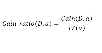
其中分裂信息：

??通俗理解??：
原始信息增益是"獎勵"，分裂信息是"懲罰"（當特征取值過多時懲罰加重）
就像公司發獎金時，既要看業績（增益），也要考慮工作難度系數（分裂信息）

4.2? 剪枝技術

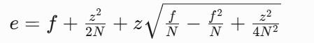
C4.5采用??悲觀錯誤剪枝(PEP)??：

計算節點誤差上限：

比較子樹和葉節點的預期誤差
當剪枝后預期誤差不增加時，剪掉子樹

?? ??剪枝哲學??：
"與其保留可能出錯的分支，不如當機立斷截肢"

4.3?代碼實現

# 使用c4.5算法
import numpy as np
import math
from collections import Counterclass Node:"""決策樹節點類（C4.5版本）"""def __init__(self, feature=None, threshold=None, value=None, results=None, children=None):self.feature = feature      # 分割特征名稱self.threshold = threshold  # 連續特征的分割閾值（僅用于連續特征）self.value = value          # 特征值（用于離散特征分支判斷）self.results = results      # 葉節點的分類結果self.children = children     # 子節點字典{特征值/區間: 節點}class C45DecisionTree:"""C4.5決策樹實現"""def __init__(self, min_samples_split=2, max_depth=5):self.min_samples_split = min_samples_split  # 最小分裂樣本數self.max_depth = max_depth                  # 樹的最大深度self.root = None                            # 決策樹根節點self.feature_types = {}                     # 存儲特征類型（離散/連續）def fit(self, data, feature_names, target_name):"""構建決策樹"""self._determine_feature_types(data, feature_names)self.root = self._build_tree(data, feature_names, target_name, depth=0)def _determine_feature_types(self, data, feature_names):"""確定特征類型（離散/連續）"""for i, name in enumerate(feature_names):# 嘗試轉換為數值，如果成功則為連續特征try:float(data[0][i])self.feature_types[name] = 'continuous'except ValueError:self.feature_types[name] = 'categorical'def _entropy(self, data):"""計算數據集的信息熵"""labels = [row[-1] for row in data]label_counts = Counter(labels)probs = [count / len(labels) for count in label_counts.values()]return -sum(p * math.log2(p) if p > 0 else 0 for p in probs)def _split_information(self, data, feature_index):"""計算特征的分裂信息（用于增益率計算）"""feature_values = [row[feature_index] for row in data]# 連續特征處理if isinstance(feature_values[0], (int, float)):return 1  # 連續特征分裂信息設為1，簡化處理# 離散特征計算分裂信息value_counts = Counter(feature_values)total = len(feature_values)return -sum((count/total) * math.log2(count/total) for count in value_counts.values())def _gain_ratio(self, data, feature_index):"""計算特征的增益率（C4.5核心改進）"""base_entropy = self._entropy(data)feature_values = [row[feature_index] for row in data]total = len(data)# 連續特征處理 - 尋找最佳分割點if isinstance(feature_values[0], (int, float)):sorted_values = sorted(set(feature_values))best_gain = 0best_threshold = None# 檢查所有可能的分割點for i in range(1, len(sorted_values)):threshold = (sorted_values[i-1] + sorted_values[i]) / 2below = [row for row in data if row[feature_index] <= threshold]above = [row for row in data if row[feature_index] > threshold]if len(below) == 0 or len(above) == 0:continuenew_entropy = (len(below)/total) * self._entropy(below) + \(len(above)/total) * self._entropy(above)gain = base_entropy - new_entropyif gain > best_gain:best_gain = gainbest_threshold = threshold# 避免除以0split_info = self._split_information(data, feature_index)return best_gain, best_threshold, best_gain / split_info if split_info > 0 else 0# 離散特征處理value_counts = Counter(feature_values)new_entropy = 0.0for value, count in value_counts.items():subset = [row for row in data if row[feature_index] == value]new_entropy += (count / total) * self._entropy(subset)gain = base_entropy - new_entropysplit_info = self._split_information(data, feature_index)return gain, None, gain / split_info if split_info > 0 else 0def _find_best_feature(self, data, feature_names):"""使用增益率尋找最佳特征"""best_gain_ratio = -1best_feature_idx = -1best_threshold = Nonefor i in range(len(data[0]) - 1):gain, threshold, gain_ratio = self._gain_ratio(data, i)# 當增益為0時跳過，避免無意義分裂if gain > 0 and gain_ratio > best_gain_ratio:best_gain_ratio = gain_ratiobest_feature_idx = ibest_threshold = thresholdreturn best_feature_idx, best_thresholddef _build_tree(self, data, feature_names, target_name, depth=0):"""遞歸構建決策樹（增加停止條件）"""# 停止條件1: 所有樣本屬于同一類別labels = [row[-1] for row in data]if len(set(labels)) == 1:return Node(results=labels[0])# 停止條件2: 無特征可用或樣本數過少if len(data[0]) == 1 or len(data) < self.min_samples_split:majority_label = Counter(labels).most_common(1)[0][0]return Node(results=majority_label)# 停止條件3: 達到最大深度if depth >= self.max_depth:majority_label = Counter(labels).most_common(1)[0][0]return Node(results=majority_label)# 選擇最佳分割特征best_feature_idx, best_threshold = self._find_best_feature(data, feature_names)# 停止條件4: 找不到合適的分裂特征if best_feature_idx == -1:majority_label = Counter(labels).most_common(1)[0][0]return Node(results=majority_label)feature_name = feature_names[best_feature_idx]children = {}# 連續特征分割if self.feature_types[feature_name] == 'continuous' and best_threshold is not None:# 創建兩個分支：小于等于閾值 和 大于閾值below = [row for row in data if row[best_feature_idx] <= best_threshold]above = [row for row in data if row[best_feature_idx] > best_threshold]children[f"≤{best_threshold:.2f}"] = self._build_tree(below, feature_names, target_name, depth+1)children[f">{best_threshold:.2f}"] = self._build_tree(above, feature_names, target_name, depth+1)return Node(feature=feature_name,threshold=best_threshold,children=children)# 離散特征分割unique_vals = {row[best_feature_idx] for row in data}for value in unique_vals:subset = [row for row in data if row[best_feature_idx] == value]if subset:  # 確保子集不為空children[value] = self._build_tree(subset, feature_names, target_name, depth+1)return Node(feature=feature_name, children=children)def predict(self, sample, feature_names):"""預測單個樣本"""node = self.rootwhile node.children is not None:feature_idx = feature_names.index(node.feature)# 連續特征處理if node.threshold is not None:if sample[feature_idx] <= node.threshold:node = node.children[f"≤{node.threshold:.2f}"]else:node = node.children[f">{node.threshold:.2f}"]# 離散特征處理else:value = sample[feature_idx]if value in node.children:node = node.children[value]else:# 處理未見過的特征值 - 使用默認子節點node = list(node.children.values())[0]return node.resultsdef print_tree(self, node=None, indent="", feature_names=None):"""打印決策樹結構（優化可讀性）"""if node is None:node = self.rootprint("決策樹結構:")if node.results is not None:print(indent + "結果:", node.results)else:# 處理連續特征顯示if node.threshold is not None:print(indent + f"特征: {node.feature} (閾值={node.threshold:.2f})")for value, child in node.children.items():print(indent + "├── 分支:", value)self.print_tree(child, indent + "│   ", feature_names)# 處理離散特征else:print(indent + f"特征: {node.feature}")children_items = list(node.children.items())for i, (value, child) in enumerate(children_items):prefix = "├──" if i < len(children_items)-1 else "└──"print(indent + prefix + " 分支:", value)self.print_tree(child, indent + ("│   " if i < len(children_items)-1 else "    "), feature_names)# 示例數據集（添加數值型特征）
# 數據集格式: [Outlook, Temperature, Humidity, WindSpeed, PlayTennis]
data = [['Sunny', 85, 85, 10, 'No'],['Sunny', 88, 90, 15, 'No'],['Overcast', 83, 86, 8, 'Yes'],['Rain', 75, 80, 5, 'Yes'],['Rain', 68, 65, 5, 'Yes'],['Rain', 65, 70, 17, 'No'],['Overcast', 64, 65, 12, 'Yes'],['Sunny', 72, 95, 6, 'No'],['Sunny', 69, 70, 5, 'Yes'],['Rain', 75, 80, 5, 'Yes'],['Sunny', 72, 60, 18, 'Yes'],['Overcast', 81, 75, 16, 'Yes'],['Overcast', 88, 60, 7, 'Yes'],['Rain', 76, 75, 15, 'No']
]feature_names = ['Outlook', 'Temperature', 'Humidity', 'WindSpeed']
target_name = 'PlayTennis'# 創建并訓練C4.5決策樹
tree = C45DecisionTree(min_samples_split=3, max_depth=3)
tree.fit(data, feature_names, target_name)# 打印決策樹
tree.print_tree()# 預測示例
sample = ['Sunny', 80, 90, 12]
prediction = tree.predict(sample, feature_names)
print(f"\n預測樣本 {sample} -> {prediction}")

決策樹結構:
特征: Humidity (閾值=88.00)
├── 分支: ≤88.00
│ ? 特征: WindSpeed (閾值=9.00)
│ ? ├── 分支: ≤9.00
│ ? │ ? 結果: Yes
│ ? ├── 分支: >9.00
│ ? │ ? 特征: Humidity (閾值=67.50)
│ ? │ ? ├── 分支: ≤67.50
│ ? │ ? │ ? 結果: Yes
│ ? │ ? ├── 分支: >67.50
│ ? │ ? │ ? 結果: No
├── 分支: >88.00
│ ? 結果: No

預測樣本 ['Sunny', 80, 90, 12] -> No

?4.4 優缺點分析

特性	ID3	C4.5
??分裂準則??	信息增益	增益率
??特征類型??	僅離散值	支持連續值
??缺失值處理??	不支持	支持缺失值（分布式處理）
??剪枝技術??	無	悲觀剪枝法
??多值特征偏好??	嚴重	有效緩解
??應用場景??	小型數據集	中等規模數據集
??計算復雜度??	低	中等（需排序連續值）
??過擬合風險??	高	中等（通過剪枝控制）

適用場景

混合型數據（連續值+離散值）
特征重要性分析
需要可視化決策邏輯的場景
中等規模數據集（<10萬條）

主要局限??：

對高維數據計算效率低
預剪枝可能導致欠擬合
內存消耗較大
多分類任務可能過于復雜

"了解C4.5，就掌握了決策樹進化的關鍵鑰匙" —— 這就是為什么它仍是機器學習課程的核心內容！

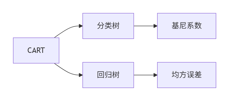
5 CarT算法

CART（Classification and Regression Trees）是既能解決分類問題又能處理回歸任務的二叉樹模型。與ID3和C4.5不同，CART有兩大革命性創新：

每個節點只做二選一決策（是/否）
即使面對多分類特征，也通過二分法處理（如"顏色=紅色?是→其他顏色?是→..."）
結構更簡單，預測路徑更清晰

5.1 分類樹

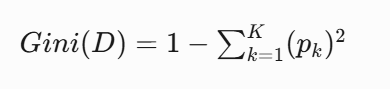
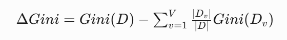
基尼系數

基尼系數（Gini Index）是決策樹（特別是CART算法）中用于衡量數據不純度（Impurity）的核心指標

基尼系數可以理解為：??隨機抽取兩個樣本，其類別不一致的概率?。想象你把不同顏色的彈珠倒進一個盒子：

如果全是紅色彈珠→基尼=0（完全純凈）
紅藍綠各占1/3→基尼=1-3×(1/3)2=0.67（高度混亂）

而CarT算法的目標：每次分裂讓盒子里的彈珠顏色盡量統一！

基尼系數公式：

??基尼增益計算??：

def gini_impurity(labels):"""計算基尼不純度"""counter = Counter(labels)impurity = 1.0for count in counter.values():prob = count / len(labels)impurity -= prob ** 2return impuritydef best_split(X, y):"""尋找最佳分割點（基于基尼系數）"""best_gain = -1best_feature = Nonebest_threshold = Nonefor feature_idx in range(X.shape[1]):# 對連續特征排序thresholds = np.unique(X[:, feature_idx])for threshold in thresholds:# 根據閾值分割數據集left_indices = X[:, feature_idx] <= thresholdright_indices = ~left_indices# 計算左右子集的基尼不純度gini_left = gini_impurity(y[left_indices])gini_right = gini_impurity(y[right_indices])# 加權平均n_left = len(y[left_indices])n_right = len(y[right_indices])weighted_gini = (n_left * gini_left + n_right * gini_right) / len(y)# 基尼增益 = 父節點不純度 - 子節點加權不純度gain = gini_impurity(y) - weighted_giniif gain > best_gain:best_gain = gainbest_feature = feature_idxbest_threshold = thresholdreturn best_feature, best_threshold

5.2 回歸樹

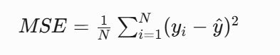
當對于連續值進行預測的時候，CART切換到回歸模式：

核心公式

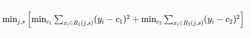
分裂策略??：

對每個特征尋找最佳切分點s
計算分裂后的樣本方差
選擇使方差減少最多的(s)：

5.3 代碼實現

# CarT算法實現
import numpy as np
import math
from collections import Counterclass Node:"""CART決策樹節點類"""def __init__(self, feature=None, threshold=None, value=None,left=None, right=None, results=None):self.feature = feature      # 分割特征名稱self.threshold = threshold  # 分割閾值（用于連續特征）self.value = value          # 特征值（用于離散特征）self.left = left            # 左子樹self.right = right          # 右子樹self.results = results      # 葉節點的結果（分類時為類別，回歸時為預測值）class CARTDecisionTree:"""CART決策樹實現（支持分類和回歸）"""def __init__(self, min_samples_split=2, max_depth=5, task='classification'):"""參數:min_samples_split: 最小分裂樣本數max_depth: 樹的最大深度task: 'classification' 或 'regression'"""self.min_samples_split = min_samples_splitself.max_depth = max_depthself.task = taskself.root = Noneself.feature_types = {}def fit(self, X, y, feature_names):"""構建決策樹"""data = np.column_stack([X, y])self._determine_feature_types(data, feature_names)self.root = self._build_tree(data, feature_names, depth=0)def _determine_feature_types(self, data, feature_names):"""確定特征類型（離散/連續）"""for i, name in enumerate(feature_names):try:float(data[0][i])self.feature_types[name] = 'continuous'except ValueError:self.feature_types[name] = 'categorical'def _calculate_impurity(self, data):"""計算不純度（基尼系數或方差）"""target_values = [row[-1] for row in data]if self.task == 'classification':# 分類任務使用基尼系數counts = Counter(target_values)impurity = 1.0for count in counts.values():prob = count / len(target_values)impurity -= prob ** 2return impurityelse:# 回歸任務使用方差mean = np.mean([float(val) for val in target_values])variance = np.mean([(float(val) - mean) ** 2 for val in target_values])return variancedef _find_best_split(self, data, feature_idx, feature_type):"""為單個特征尋找最佳分割點"""best_gain = -float('inf')best_threshold = Nonebest_left_indices = Nonebest_right_indices = Nonevalues = [row[feature_idx] for row in data]target_values = [row[-1] for row in data]if feature_type == 'continuous':# 連續特征處理unique_vals = sorted(set(float(val) for val in values))# 檢查所有可能的分割點for i in range(1, len(unique_vals)):threshold = (unique_vals[i-1] + unique_vals[i]) / 2left_indices = []right_indices = []for j, val in enumerate(values):if float(val) <= threshold:left_indices.append(j)else:right_indices.append(j)if not left_indices or not right_indices:continue# 計算不純度減少量gain = self._calculate_split_gain(data, left_indices, right_indices, target_values)if gain > best_gain:best_gain = gainbest_threshold = thresholdbest_left_indices = left_indicesbest_right_indices = right_indiceselse:# 離散特征處理（二值分裂）unique_vals = set(values)for val in unique_vals:left_indices = []right_indices = []for j, v in enumerate(values):if v == val:left_indices.append(j)else:right_indices.append(j)if not left_indices or not right_indices:continue# 計算不純度減少量gain = self._calculate_split_gain(data, left_indices, right_indices, target_values)if gain > best_gain:best_gain = gainbest_threshold = valbest_left_indices = left_indicesbest_right_indices = right_indicesreturn best_gain, best_threshold, best_left_indices, best_right_indicesdef _calculate_split_gain(self, data, left_indices, right_indices, target_values):"""計算分裂帶來的不純度減少量"""n = len(data)n_left = len(left_indices)n_right = len(right_indices)# 計算父節點的不純度parent_impurity = self._calculate_impurity(data)# 獲取左右子樹的數據left_data = [data[i] for i in left_indices]right_data = [data[i] for i in right_indices]# 計算左右子樹的不純度left_impurity = self._calculate_impurity(left_data)right_impurity = self._calculate_impurity(right_data)# 計算加權平均不純度weighted_impurity = (n_left / n) * left_impurity + (n_right / n) * right_impurity# 增益 = 父節點不純度 - 子節點加權不純度return parent_impurity - weighted_impuritydef _find_best_split_feature(self, data, feature_names):"""尋找最佳分裂特征和分割點"""best_gain = -float('inf')best_feature_idx = Nonebest_threshold = Nonebest_left_indices = Nonebest_right_indices = Nonefor i, name in enumerate(feature_names):feature_type = self.feature_types[name]gain, threshold, left_indices, right_indices = self._find_best_split(data, i, feature_type)if gain > best_gain:best_gain = gainbest_feature_idx = ibest_threshold = thresholdbest_left_indices = left_indicesbest_right_indices = right_indicesreturn best_feature_idx, best_threshold, best_left_indices, best_right_indicesdef _build_tree(self, data, feature_names, depth=0):"""遞歸構建決策樹"""# 停止條件1: 所有樣本目標值相同target_values = [row[-1] for row in data]if len(set(target_values)) == 1:return Node(results=target_values[0])# 停止條件2: 達到最大深度或樣本數不足if depth >= self.max_depth or len(data) < self.min_samples_split:return self._create_leaf_node(data)# 尋找最佳分割點best_feature_idx, best_threshold, left_indices, right_indices = self._find_best_split_feature(data, feature_names)# 如果找不到有效的分裂點if best_feature_idx is None or left_indices is None or right_indices is None:return self._create_leaf_node(data)# 獲取左右子樹的數據left_data = [data[i] for i in left_indices]right_data = [data[i] for i in right_indices]# 創建當前節點node = Node(feature=feature_names[best_feature_idx],threshold=best_threshold,left=self._build_tree(left_data, feature_names, depth+1),right=self._build_tree(right_data, feature_names, depth+1))return nodedef _create_leaf_node(self, data):"""創建葉節點（根據任務類型返回不同結果）"""target_values = [row[-1] for row in data]if self.task == 'classification':# 分類任務：返回多數類別most_common = Counter(target_values).most_common(1)return Node(results=most_common[0][0])else:# 回歸任務：返回平均值return Node(results=np.mean([float(val) for val in target_values]))def predict(self, sample, feature_names):"""預測單個樣本"""return self._traverse_tree(sample, self.root, feature_names)def _traverse_tree(self, sample, node, feature_names):"""遞歸遍歷決策樹進行預測"""# 到達葉節點if node.results is not None:return node.results# 獲取特征索引feature_idx = feature_names.index(node.feature)# 根據特征類型處理if self.feature_types[node.feature] == 'continuous':# 連續特征：與閾值比較if float(sample[feature_idx]) <= float(node.threshold):return self._traverse_tree(sample, node.left, feature_names)else:return self._traverse_tree(sample, node.right, feature_names)else:# 離散特征：檢查是否等于閾值if sample[feature_idx] == node.threshold:return self._traverse_tree(sample, node.left, feature_names)else:return self._traverse_tree(sample, node.right, feature_names)def print_tree(self, node=None, indent="", feature_names=None):"""打印決策樹結構"""if node is None:node = self.rootprint("CART決策樹結構:")if node.results is not None:print(indent + "結果:", node.results)else:if self.feature_types[node.feature] == 'continuous':print(indent + f"特征: {node.feature} (閾值={node.threshold:.2f})")else:print(indent + f"特征: {node.feature} (值={node.threshold})")print(indent + "├── 左子樹:")self.print_tree(node.left, indent + "│   ", feature_names)print(indent + "└── 右子樹:")self.print_tree(node.right, indent + "    ", feature_names)# 分類任務示例
print("==== 分類任務示例 ====")
# 數據集格式: [Outlook, Temperature, Humidity, WindSpeed, PlayTennis]
X = [['Sunny', 85, 85, 10],['Sunny', 88, 90, 15],['Overcast', 83, 86, 8],['Rain', 75, 80, 5],['Rain', 68, 65, 5],['Rain', 65, 70, 17],['Overcast', 64, 65, 12],['Sunny', 72, 95, 6],['Sunny', 69, 70, 5],['Rain', 75, 80, 5],['Sunny', 72, 60, 18],['Overcast', 81, 75, 16],['Overcast', 88, 60, 7],['Rain', 76, 75, 15]
]
y = ['No', 'No', 'Yes', 'Yes', 'Yes', 'No', 'Yes', 'No', 'Yes', 'Yes', 'Yes', 'Yes', 'Yes', 'No']
feature_names = ['Outlook', 'Temperature', 'Humidity', 'WindSpeed']# 創建并訓練CART分類樹
class_tree = CARTDecisionTree(min_samples_split=3, max_depth=3, task='classification')
class_tree.fit(X, y, feature_names)# 打印決策樹
class_tree.print_tree(feature_names=feature_names)# 預測示例
sample = ['Sunny', 80, 90, 12]
prediction = class_tree.predict(sample, feature_names)
print(f"\n預測樣本 {sample} -> {prediction}")# 回歸任務示例
print("\n==== 回歸任務示例 ====")
# 房價預測數據集: [房間數, 面積(m2), 房齡(年), 房價(萬元)]
X = [[3, 85, 10],[4, 88, 5],[2, 83, 20],[3, 75, 15],[4, 68, 8],[3, 65, 25],[3, 64, 18],[2, 72, 10],[1, 69, 30],[4, 75, 5],[3, 72, 12],[5, 81, 7],[3, 88, 3],[2, 76, 22]
]
y = [200, 240, 180, 190, 210, 175, 170, 185, 150, 250, 195, 280, 270, 165]
feature_names = ['房間數', '面積', '房齡']# 創建并訓練CART回歸樹
reg_tree = CARTDecisionTree(min_samples_split=2, max_depth=4, task='regression')
reg_tree.fit(X, y, feature_names)# 打印決策樹
reg_tree.print_tree(feature_names=feature_names)# 預測示例
sample = [3, 80, 12]
prediction = reg_tree.predict(sample, feature_names)
print(f"\n預測樣本 {sample} -> 房價: {prediction:.2f}萬元")

==== 分類任務示例 ====
CART決策樹結構:
特征: Humidity (閾值=88.00)
├── 左子樹:
│ ? 特征: WindSpeed (閾值=9.00)
│ ? ├── 左子樹:
│ ? │ ? 結果: Yes
│ ? └── 右子樹:
│ ? ? ? 特征: Outlook (值=Overcast)
│ ? ? ? ├── 左子樹:
│ ? ? ? │ ? 結果: Yes
│ ? ? ? └── 右子樹:
│ ? ? ? ? ? 結果: No
└── 右子樹:
結果: No

預測樣本 ['Sunny', 80, 90, 12] -> No

==== 回歸任務示例 ====
CART決策樹結構:
特征: 房齡 (閾值=7.50)
├── 左子樹:
│ ? 特征: 房間數 (閾值=4.50)
│ ? ├── 左子樹:
│ ? │ ? 特征: 房間數 (閾值=3.50)
│ ? │ ? ├── 左子樹:
│ ? │ ? │ ? 結果: 270
│ ? │ ? └── 右子樹:
│ ? │ ? ? ? 特征: 面積 (閾值=81.50)
│ ? │ ? ? ? ├── 左子樹:
│ ? │ ? ? ? │ ? 結果: 250
│ ? │ ? ? ? └── 右子樹:
│ ? │ ? ? ? ? ? 結果: 240
│ ? └── 右子樹:
│ ? ? ? 結果: 280
└── 右子樹:
特征: 房齡 (閾值=16.50)
├── 左子樹:
│ ? 特征: 房間數 (閾值=3.50)
│ ? ├── 左子樹:
│ ? │ ? 特征: 房間數 (閾值=2.50)
│ ? │ ? ├── 左子樹:
│ ? │ ? │ ? 結果: 185
│ ? │ ? └── 右子樹:
│ ? │ ? ? ? 結果: 195.0
│ ? └── 右子樹:
│ ? ? ? 結果: 210
└── 右子樹:
特征: 房間數 (閾值=1.50)
├── 左子樹:
│ ? 結果: 150
└── 右子樹:
特征: 面積 (閾值=79.50)
├── 左子樹:
│ ? 結果: 170.0
└── 右子樹:
結果: 180

預測樣本 [3, 80, 12] -> 房價: 195.00萬元

5.4?優缺點分析

核心優勢??：

1. 雙重任務能力業界唯一同時支持分類和回歸的決策樹?統一框架簡化模型選型

2. 二叉樹效率革命決策路徑復雜度：O(log?n) vs 其他決策樹的O(n) 更快的預測速度

3. 優秀的剪枝機制? 代價復雜度剪枝有效控制過擬合懲罰系數α提供精細調節

4. 特征處理全能王?自動處理連續/離散特征無縮放要求，魯棒性強

??主要局限??：

1. 二元分裂限制對多分類特征需要多次分裂可能創建冗余分支

2. 貪心算法缺陷局部最優但不保證全局最優對分裂順序敏感

3. 高方差問題??小數據集易過擬合需依賴剪枝和集成方法

4. 解釋性折衷? 比單棵樹的邏輯回歸難解釋多路徑分析復雜

6 案例使用

信用卡欺詐檢測

下面是一個完整的信用卡欺詐檢測案例，使用決策樹算法識別可疑交易。該案例包含詳細的數據預處理、模型訓練、評估和可視化步驟。

import numpy as np
import pandas as pd
import matplotlib.pyplot as plt
import seaborn as sns
from sklearn.model_selection import train_test_split, GridSearchCV
from sklearn.preprocessing import StandardScaler
from sklearn.tree import DecisionTreeClassifier, plot_tree
from sklearn.metrics import (confusion_matrix, classification_report,roc_auc_score, roc_curve, precision_recall_curve,average_precision_score)
from sklearn.utils import resample
from imblearn.over_sampling import SMOTE
import warnings
warnings.filterwarnings('ignore')# 1. 數據加載與探索
# 數據集來源：Kaggle信用卡欺詐檢測數據集（已脫敏）
# https://www.kaggle.com/mlg-ulb/creditcardfraud# 加載數據
df = pd.read_csv('creditcard.csv')  # 請確保文件路徑正確print("數據集維度:", df.shape)
print("\n前5行數據:")
print(df.head())# 檢查數據分布
print("\n類別分布:")
print(df['Class'].value_counts(normalize=True))# 可視化類別分布
plt.figure(figsize=(10, 6))
sns.countplot(x='Class', data=df)
plt.title('交易類別分布 (0:正常, 1:欺詐)')
plt.show()# 2. 數據預處理
# 檢查缺失值
print("\n缺失值統計:")
print(df.isnull().sum().max())  # 該數據集沒有缺失值# 特征和時間處理
# 將Time特征轉換為小時
df['Hour'] = df['Time'].apply(lambda x: divmod(x, 3600)[0])
df.drop(['Time'], axis=1, inplace=True)# 對Amount進行標準化
scaler = StandardScaler()
df['Amount'] = scaler.fit_transform(df['Amount'].values.reshape(-1, 1))# 分離特征和標簽
X = df.drop('Class', axis=1)
y = df['Class']# 3. 處理類別不平衡
# 欺詐交易僅占0.17%，需要處理不平衡問題# 方法1：下采樣多數類
# normal = df[df.Class == 0]
# fraud = df[df.Class == 1]
# normal_downsampled = resample(normal,
#                              replace=False,
#                              n_samples=len(fraud),
#                              random_state=42)
# df_downsampled = pd.concat([normal_downsampled, fraud])
# X_down = df_downsampled.drop('Class', axis=1)
# y_down = df_downsampled['Class']# 方法2：使用SMOTE過采樣少數類（效果更好）
smote = SMOTE(random_state=42)
X_res, y_res = smote.fit_resample(X, y)print("\n過采樣后類別分布:")
print(pd.Series(y_res).value_counts(normalize=True))# 4. 劃分訓練集和測試集
X_train, X_test, y_train, y_test = train_test_split(X_res, y_res, test_size=0.2, random_state=42, stratify=y_res
)print("\n訓練集維度:", X_train.shape)
print("測試集維度:", X_test.shape)# 5. 決策樹模型訓練
# 創建基礎決策樹模型
base_dt = DecisionTreeClassifier(random_state=42)
base_dt.fit(X_train, y_train)# 模型評估函數
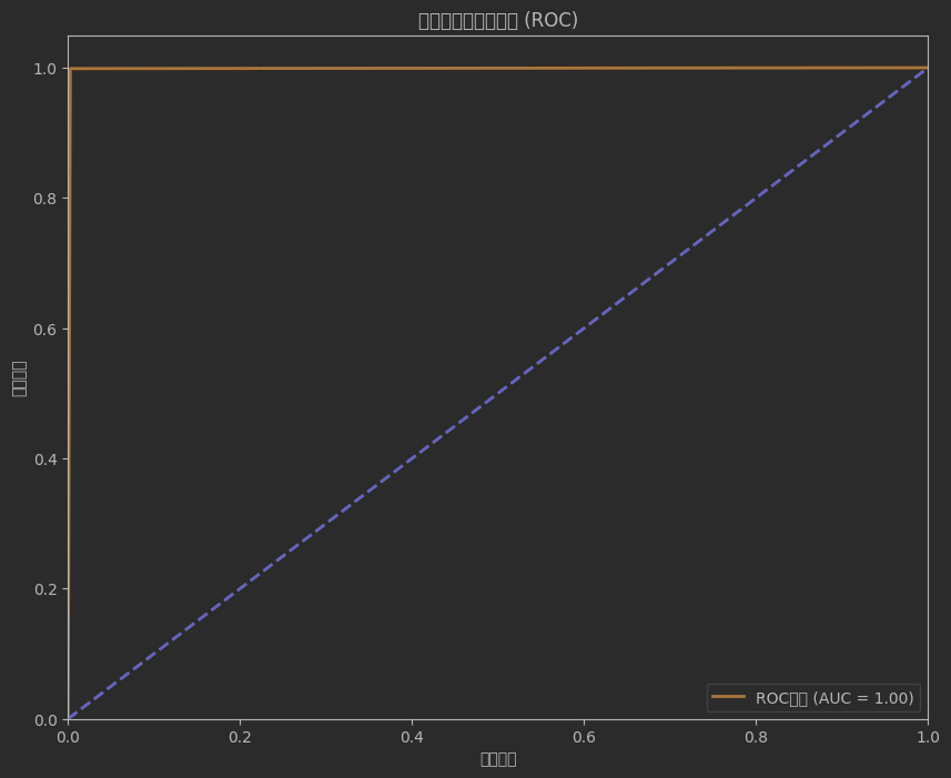
def evaluate_model(model, X_test, y_test):"""評估模型性能并生成報告"""y_pred = model.predict(X_test)y_prob = model.predict_proba(X_test)[:, 1]# 混淆矩陣cm = confusion_matrix(y_test, y_pred)plt.figure(figsize=(8, 6))sns.heatmap(cm, annot=True, fmt='d', cmap='Blues',xticklabels=['正常', '欺詐'],yticklabels=['正常', '欺詐'])plt.xlabel('預測值')plt.ylabel('真實值')plt.title('混淆矩陣')plt.show()# 分類報告print("\n分類報告:")print(classification_report(y_test, y_pred, target_names=['正常', '欺詐']))# ROC曲線fpr, tpr, thresholds = roc_curve(y_test, y_prob)roc_auc = roc_auc_score(y_test, y_prob)plt.figure(figsize=(10, 8))plt.plot(fpr, tpr, color='darkorange', lw=2, label=f'ROC曲線 (AUC = {roc_auc:.2f})')plt.plot([0, 1], [0, 1], color='navy', lw=2, linestyle='--')plt.xlim([0.0, 1.0])plt.ylim([0.0, 1.05])plt.xlabel('假陽性率')plt.ylabel('真陽性率')plt.title('受試者工作特征曲線 (ROC)')plt.legend(loc="lower right")plt.show()# 精確率-召回率曲線precision, recall, _ = precision_recall_curve(y_test, y_prob)avg_precision = average_precision_score(y_test, y_prob)plt.figure(figsize=(10, 8))plt.plot(recall, precision, color='blue', lw=2,label=f'PR曲線 (AP = {avg_precision:.2f})')plt.xlabel('召回率')plt.ylabel('精確率')plt.title('精確率-召回率曲線')plt.legend(loc="upper right")plt.show()return roc_auc, avg_precision# 評估基礎模型
print("基礎決策樹模型性能:")
base_roc_auc, base_ap = evaluate_model(base_dt, X_test, y_test)# 6. 模型優化 - 網格搜索調參
param_grid = {'max_depth': [5, 10, 15, 20, None],'min_samples_split': [2, 5, 10],'min_samples_leaf': [1, 2, 4],'criterion': ['gini', 'entropy'],'max_features': ['sqrt', 'log2', None]
}grid_dt = GridSearchCV(DecisionTreeClassifier(random_state=42),param_grid=param_grid,cv=5,scoring='roc_auc',n_jobs=-1,verbose=1
)grid_dt.fit(X_train, y_train)# 最佳參數
print("\n最佳參數:")
print(grid_dt.best_params_)# 使用最佳參數的模型
best_dt = grid_dt.best_estimator_# 評估優化后的模型
print("\n優化后決策樹模型性能:")
best_roc_auc, best_ap = evaluate_model(best_dt, X_test, y_test)# 7. 特征重要性分析
# 獲取特征重要性
feature_importances = best_dt.feature_importances_
feature_names = X_train.columns# 創建特征重要性DataFrame
feature_imp_df = pd.DataFrame({'Feature': feature_names,'Importance': feature_importances
}).sort_values('Importance', ascending=False)# 可視化特征重要性
plt.figure(figsize=(12, 8))
sns.barplot(x='Importance', y='Feature', data=feature_imp_df.head(15))
plt.title('Top 15 特征重要性')
plt.xlabel('重要性')
plt.ylabel('特征')
plt.show()# 8. 決策樹可視化
plt.figure(figsize=(20, 12))
plot_tree(best_dt,max_depth=3,  # 限制深度以便可視化feature_names=feature_names,class_names=['正常', '欺詐'],filled=True,rounded=True,proportion=True
)
plt.title('決策樹結構 (前3層)')
plt.show()# 9. 在原始不平衡數據上評估模型
# 注意：我們使用原始測試集（未過采樣）
y_pred_orig = best_dt.predict(X_test_orig)
y_prob_orig = best_dt.predict_proba(X_test_orig)[:, 1]# 計算欺詐檢測的關鍵指標
tn, fp, fn, tp = confusion_matrix(y_test_orig, y_pred_orig).ravel()print("\n在原始不平衡測試集上的性能:")
print(f"準確率: {(tp+tn)/(tp+tn+fp+fn):.4f}")
print(f"精確率: {tp/(tp+fp):.4f}")
print(f"召回率: {tp/(tp+fn):.4f}")
print(f"F1分數: {2*tp/(2*tp+fp+fn):.4f}")
print(f"AUC: {roc_auc_score(y_test_orig, y_prob_orig):.4f}")# 10. 業務應用 - 設置閾值優化
# 尋找最佳閾值以平衡精確率和召回率
precisions, recalls, thresholds = precision_recall_curve(y_test_orig, y_prob_orig)# 計算F1分數
f1_scores = 2 * (precisions * recalls) / (precisions + recalls + 1e-8)# 找到最佳閾值（最大化F1分數）
best_idx = np.argmax(f1_scores)
best_threshold = thresholds[best_idx]
best_f1 = f1_scores[best_idx]print(f"\n最佳閾值: {best_threshold:.4f}")
print(f"最佳F1分數: {best_f1:.4f}")# 使用最佳閾值進行預測
y_pred_thresh = (y_prob_orig >= best_threshold).astype(int)# 混淆矩陣
cm_thresh = confusion_matrix(y_test_orig, y_pred_thresh)
plt.figure(figsize=(8, 6))
sns.heatmap(cm_thresh, annot=True, fmt='d', cmap='Blues',xticklabels=['正常', '欺詐'],yticklabels=['正常', '欺詐'])
plt.xlabel('預測值')
plt.ylabel('真實值')
plt.title('使用最佳閾值的混淆矩陣')
plt.show()# 11. 模型部署建議
print("\n模型部署建議:")
print("1. 在實時交易系統中集成模型預測功能")
print("2. 當模型預測為欺詐時，觸發人工審核流程")
print("3. 設置動態閾值調整機制，根據業務需求平衡誤報率和漏報率")
print("4. 定期（每周/每月）重新訓練模型以適應數據分布變化")
print("5. 監控模型性能指標，特別是欺詐類別的召回率")# 12. 保存模型
import joblibjoblib.dump(best_dt, 'credit_card_fraud_detection_model.pkl')
print("\n模型已保存為 'credit_card_fraud_detection_model.pkl'")

數據集維度: (284807, 31)
前5行數據:
Time ? ? ? ?V1 ? ? ? ?V2 ? ? ? ?V3 ? ? ? ?V4 ? ? ? ?V5 ? ? ? ?V6 ? ? ? ?V7 ?\
0 ? 0.0 -1.359807 -0.072781 ?2.536347 ?1.378155 -0.338321 ?0.462388 ?0.239599 ??
1 ? 0.0 ?1.191857 ?0.266151 ?0.166480 ?0.448154 ?0.060018 -0.082361 -0.078803 ??
2 ? 1.0 -1.358354 -1.340163 ?1.773209 ?0.379780 -0.503198 ?1.800499 ?0.791461 ??
3 ? 1.0 -0.966272 -0.185226 ?1.792993 -0.863291 -0.010309 ?1.247203 ?0.237609 ??
4 ? 2.0 -1.158233 ?0.877737 ?1.548718 ?0.403034 -0.407193 ?0.095921 ?0.592941 ??
? ? ? ? ?V8 ? ? ? ?V9 ?... ? ? ? V21 ? ? ? V22 ? ? ? V23 ? ? ? V24 ? ? ? V25 ?\
0 ?0.098698 ?0.363787 ?... -0.018307 ?0.277838 -0.110474 ?0.066928 ?0.128539 ??
1 ?0.085102 -0.255425 ?... -0.225775 -0.638672 ?0.101288 -0.339846 ?0.167170 ??
2 ?0.247676 -1.514654 ?... ?0.247998 ?0.771679 ?0.909412 -0.689281 -0.327642 ??
3 ?0.377436 -1.387024 ?... -0.108300 ?0.005274 -0.190321 -1.175575 ?0.647376 ??
4 -0.270533 ?0.817739 ?... -0.009431 ?0.798278 -0.137458 ?0.141267 -0.206010 ??
? ? ? ? V26 ? ? ? V27 ? ? ? V28 ?Amount ?Class ?
0 -0.189115 ?0.133558 -0.021053 ?149.62 ? ? ?0 ?
1 ?0.125895 -0.008983 ?0.014724 ? ?2.69 ? ? ?0 ?
2 -0.139097 -0.055353 -0.059752 ?378.66 ? ? ?0 ?
3 -0.221929 ?0.062723 ?0.061458 ?123.50 ? ? ?0 ?
4 ?0.502292 ?0.219422 ?0.215153 ? 69.99 ? ? ?0 ?
[5 rows x 31 columns]
類別分布:
Class
0 ? ?0.998273
1 ? ?0.001727
Name: proportion, dtype: float64