任務

實戰（二）：MLP 實現圖像多分類
基于 mnist 數據集，建立 mlp 模型，實現 0-9 數字的十分類 task:
1、實現 mnist 數據載入，可視化圖形數字；
2、完成數據預處理：圖像數據維度轉換與歸一化、輸出結果格式轉換；
3、計算模型在預測數據集的準確率；
4、模型結構：兩層隱藏層，每層有 392 個神經元

參考資料

38.42 實戰（二）_嗶哩嗶哩_bilibili

?1、載入mnist 數據，可視化圖形數字

載入數據

#load the mnist data
from tensorflow.keras.datasets import mnist
(X_train, y_train),(X_test, y_test) = mnist.load_data()

print(type(X_train), X_train.shape) 
#<class 'numpy.ndarray'> (60000, 28, 28)，訓練樣本有 60000個，每個都是 28 * 28 像素組成的 Array

可視化部分數據

#可視化部分數據
img1 = X_train[0] #取第一個數據
%matplotlib inline
from matplotlib import pyplot as plt
fig1 = plt.figure(figsize=(3,3))
plt.imshow(img1)
plt.title(y_train[0])# 標簽作為 title
plt.show()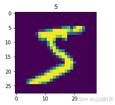

?2、數據預處理

圖像數據維度轉換與歸一化

img1.shape# (28,28), 可以看出是  28 行 28 列
#需要轉換成 784列的新的數組

#format the input data
feature_size = img1.shape[0] * img1.shape[1] # 行數*列數
print(feature_size)# 784
#把原來的數據進行 reshape
X_train_format = X_train.reshape(X_train.shape[0], feature_size)#第一個參數是樣本數量
print(X_train_format.shape)# (60000, 784), 60000個樣本， 784列X_test_format = X_test.reshape(X_test.shape[0], feature_size)#第一個參數是樣本數量
print(X_test_format.shape)#(10000, 784)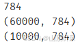

#歸一化：圖像數據是 0-255，區間太大，需要歸一化到 0-1之間
#normalize the input data
X_train_normal = X_train_format/255
X_test_normal = X_test_format/255
print(X_train_format[0]) #原數據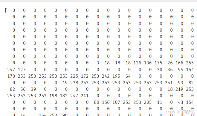

print(X_train_normal[0]) #歸一化后的數據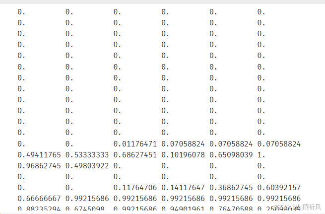

?輸出結果格式轉換

#數據預處理：輸出結果也需要進行轉換，轉換成 0001這樣的標簽
#format the output data(labels)
from tensorflow.keras.utils import to_categorical
y_train_format = to_categorical(y_train)
y_test_format = to_categorical(y_test)
print(y_train[0])# 5, 第一副圖像是 5
print(y_train_format[0])#[0. 0. 0. 0. 0. 1. 0. 0. 0. 0.] # 第 5 個是 1

3、計算模型在預測數據集的準確率

創建 MLP 模型

# set up the model
from tensorflow.keras.models import Sequential
from tensorflow.keras.layers import Dense, Activationmlp =Sequential()
mlp.add(Dense(units = 392, activation = 'sigmoid', input_dim = feature_size))
#第二層有 392 個神經元，input_dim 為一開始的輸入數據
mlp.add(Dense(units = 392, activation = 'sigmoid'))# 第三層
mlp.add(Dense(units = 10, activation = 'softmax')) # 輸出層為0-9 10個數字
mlp.summary()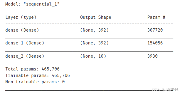

配置模型?

#config the model
mlp.compile(loss = 'categorical_crossentropy' , optimizer = 'adam')
#categorial_crossentropy: 這個是用于多分類的損失函數； optimizer:優化方法

?訓練模型

#train the model
mlp.fit(X_train_normal, y_train_format, epochs = 10)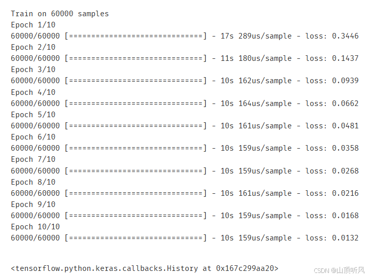

評估模型?

訓練集

#預測訓練集數據
y_train_predict = mlp.predict_classes(X_train_normal)
print(y_train_predict)

#計算對訓練集預測的準確率
from sklearn.metrics import accuracy_score
accuracy_train = accuracy_score(y_train, y_train_predict)
print(accuracy_train)#0.9964833333333334

測試集

#看下 測試集 的準確率
y_test_predict = mlp.predict_classes(X_test_normal)
accuracy_test = accuracy_score(y_test, y_test_predict)
print(accuracy_test)#0.981, 比較高，說明模型對圖片的預測還是比較準確的

展示出圖形，看預測結果與實際是否相符

#選幾幅圖展示出來，看看預測結果是否一樣
img2 = X_test[100] # 隨便選擇，這里選擇第 11 幅圖
fig2 = plt.figure(figsize = (3,3))
plt.imshow(img2)
plt.title(y_test_predict[100])
plt.show()#展示的是測試集第 11 張圖片的圖形 以及 預測的標簽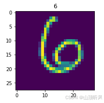

4、圖像數字多分類實戰總結

1、通過 mlp 模型，實現了基于圖像數據的數字自動識別分類；
2、完成了圖像的數字化處理與可視化；
3、對 mlp 模型的輸入、輸出數據格式有了更深的認識，完成了數據預處理與格式轉換；
4、建立了結構更為復雜的 mlp 模型
5、mnist 數據集地址：http://yann.lecun.com/exdb/mnist/