1.LeNet-5?神經網絡

以下是針對?LeNet-5?神經網絡的詳細參數解析和圖片尺寸變化分析，和原始論文設計，通過分步計算說明各層的張量變換過程。

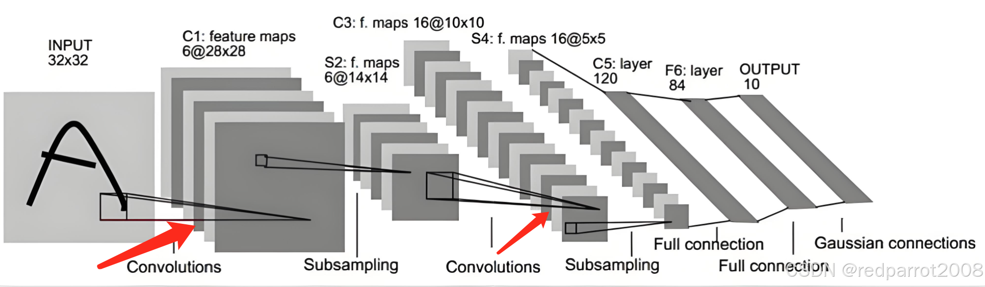
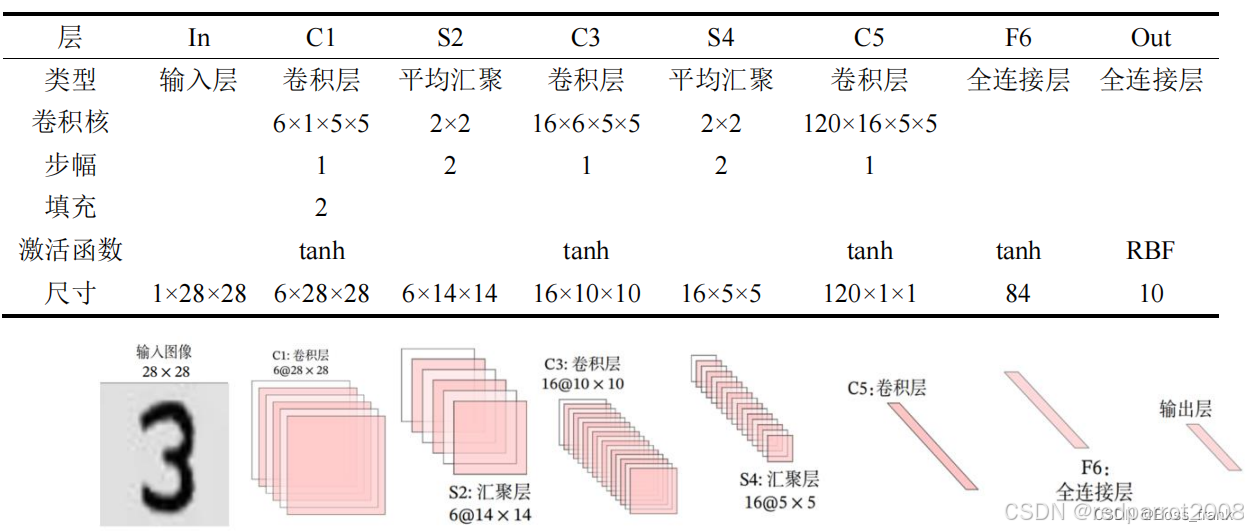
經典的 LeNet-5架構簡化版（原始論文輸入為 32x32，MNIST 常用 28x28 需調整）。完整結構如下：

• 網絡結構：
  輸入 → Conv1 → 激活/池化 → Conv2 → 激活/池化 → 展平 → FC1 → FC2 → FC3 → 輸出

• 適用場景：
  經典的小型 CNN，適合處理低分辨率圖像分類任務（如 MNIST、CIFAR-10）。

class LeNet5(nn.Module):def __init__(self):super(LeNet5, self).__init__()self.conv1 = nn.Conv2d(1, 6, 5)      # C1: 輸入1通道，輸出6通道，5x5卷積self.pool1 = nn.AvgPool2d(2, 2)       # S2: 2x2平均池化self.conv2 = nn.Conv2d(6, 16, 5)     # C3: 輸入6，輸出16，5x5卷積self.pool2 = nn.AvgPool2d(2, 2)       # S4: 2x2平均池化self.fc1 = nn.Linear(16*5*5, 120)    # C5: 全連接層self.fc2 = nn.Linear(120, 84)        # F6: 全連接層self.fc3 = nn.Linear(84, 10)         # 輸出層def forward(self, x):x = F.relu(self.conv1(x))  # 卷積 + ReLU 激活x = F.max_pool2d(x, 2)      # 2x2 最大池化x = F.relu(self.conv2(x))x = F.max_pool2d(x, 2)x = x.view(-1, 16*5*5)      # 展平特征圖x = F.relu(self.fc1(x))x = F.relu(self.fc2(x))x = self.fc3(x)             # 輸出層（通常不加激活函數）return x

1.2. 定義卷積層

定義
輸入通道是指輸入數據中獨立的“特征平面”數量。對于圖像數據，通常對應顏色通道或上一層的特征圖數量。

self.conv1 = nn.Conv2d(1, 6, 5) ? ?# 第一層卷積
self.conv2 = nn.Conv2d(6, 16, 5) ? # 第二層卷積nn.Conv2d 參數說明conv1:
輸入通道數 1（適用于單通道灰度圖，如 MNIST）。
輸出通道數 6（即 6 個卷積核，提取 6 種特征）。
卷積核大小 5x5。conv2:
輸入通道數 6（與 conv1 的輸出一致）。
輸出通道數 16（更深層的特征映射）。
卷積核大小 5x5。作用
通過卷積操作提取圖像的空間特征（如邊緣、紋理等），通道數的增加意味著學習更復雜的特征組合。每個輸出通道由一組卷積核生成：
如果輸出通道數為?6，則會有?6?個不同的卷積核（每個核的尺寸為?5x5，在單輸入通道下），分別提取不同的特征。輸出通道的維度：
輸出數據的形狀為?(batch_size, output_channels, height, width)。例如：
nn.Conv2d(3, 16, 5)  # 輸入通道=3（RGB），輸出通道=16
該層會使用?16?個卷積核，每個核的尺寸為?5x5x3（因為輸入有 3 通道）。每個核在輸入數據上滑動計算，生成 1 個輸出通道的特征圖，最終得到 16 個特征圖。

?1.3定義全連接層

self.fc1 = nn.Linear(16*5*5, 120)  # 第一個全連接層
self.fc2 = nn.Linear(120, 84)      # 第二個全連接層
self.fc3 = nn.Linear(84, 10)       # 輸出層nn.Linear 參數說明fc1:
輸入維度 16*5*5（假設卷積后特征圖尺寸為 5x5，共 16 個通道，展平后為 400 維）。
輸出維度 120（隱藏層神經元數量）。fc2:
輸入維度 120，輸出維度 84（進一步壓縮特征）。fc3:
輸入維度 84，輸出維度 10（對應 10 個分類類別，如數字 0~9）。作用
將卷積層提取的二維特征展平為一維向量，通過全連接層進行非線性變換，最終映射到分類結果。

2. 參數解析（以輸入?32x32?為例）

(1) 卷積層參數計算

• 公式：
  參數量 =?(kernel_height × kernel_width × input_channels + 1) ×output_channels
  （+1?為偏置項）

層名	參數定義	參數量計算	結果
C1	nn.Conv2d(1, 6, 5)	(5×5×1 + 1)×6	156
C3	nn.Conv2d(6, 16, 5)	(5×5×6 + 1)×16	2416

(2) 全連接層參數計算

• 公式：
  參數量 =?(input_features + 1) × output_features

層名	參數定義	參數量計算	結果
C5	nn.Linear(16*5*5, 120)	(400 + 1)×120	48120
F6	nn.Linear(120, 84)	(120 + 1)×84	10164
輸出	nn.Linear(84, 10)	(84 + 1)×10	850

總參數量：156 + 2416 + 48120 + 10164 + 850 = 61,706

3. 圖片尺寸解析（輸入?32x32）

(1) 尺寸變化公式

• 卷積層：
  H_out = floor((H_in + 2×padding - kernel_size) / stride + 1)
  （默認?stride=1,?padding=0）

• 池化層：
  H_out = floor((H_in - kernel_size) / stride + 1)
  （通常?stride=kernel_size）

(2) 逐層尺寸變化

層名	操作類型	參數	輸入尺寸	輸出尺寸計算	結果
輸入	-	-	1×32×32	-	1×32×32
C1	卷積	kernel=5, stride=1	1×32×32	(32 - 5)/1 + 1 = 28	6×28×28
S2	平均池化	kernel=2, stride=2	6×28×28	(28 - 2)/2 + 1 = 14	6×14×14
C3	卷積	kernel=5, stride=1	6×14×14	(14 - 5)/1 + 1 = 10	16×10×10
S4	平均池化	kernel=2, stride=2	16×10×10	(10 - 2)/2 + 1 = 5	16×5×5
C5	展平+全連接	-	16×5×5	展平為 400 維向量	120
F6	全連接	-	120	-	84
輸出	全連接	-	84	-	10

(3) 關鍵問題解答

Q1: 為什么全連接層?fc1?的輸入是?16*5*5？

• 經過兩次卷積和池化后，特征圖尺寸從?32x32?→?28x28?→?14x14?→?10x10?→?5x5，且最后一層有 16 個通道，因此展平后的維度為?16×5×5=400。

Q2: 如果輸入是?28x28（如 MNIST），尺寸會如何變化？

• 調整方式：
  修改第一層卷積的?padding=2（在四周補零），使輸出尺寸滿足?(28+4-5)/1 +1=28（保持尺寸不變），后續計算與原始 LeNet-5 一致。

  self.conv1 = nn.Conv2d(1, 6, 5, padding=2) # 保持28x28

  Q3: 參數量主要集中在哪部分？

• 全連接層?C5?占總數 78% (48120/61706)，這是 LeNet-5 的設計瓶頸。現代 CNN 通常用全局平均池化（GAP）替代全連接層以減少參數。

5. 完整尺寸變換流程圖（輸入?32x32）

輸入: 1×32×32 ↓ [C1] Conv2d(1,6,5)
6×28×28 ↓ [S2] AvgPool2d(2,2)
6×14×14 ↓ [C3] Conv2d(6,16,5)
16×10×10 ↓ [S4] AvgPool2d(2,2)
16×5×5 ↓ 展平
400 ↓ [C5] Linear(400,120)
120 ↓ [F6] Linear(120,84)
84 ↓ 輸出
10

?使用下面代碼，可以看到具體參數量：

# 遍歷模型的所有子模塊
for name, param in model.named_parameters():if param.requires_grad:print(f"Layer: {name}")if 'weight' in name:print(f"Weights:{param.data.shape}")if 'bias' in name:print(f"Bias:{param.data.shape}\n")

?輸出：

Layer: feature_extractor.0.weight
Weights:torch.Size([6, 1, 5, 5])
Layer: feature_extractor.0.bias
Bias:torch.Size([6])Layer: feature_extractor.2.weight
Weights:torch.Size([16, 6, 5, 5])
Layer: feature_extractor.2.bias
Bias:torch.Size([16])Layer: classifier.1.weight
Weights:torch.Size([120, 400])
Layer: classifier.1.bias
Bias:torch.Size([120])Layer: classifier.2.weight
Weights:torch.Size([84, 120])
Layer: classifier.2.bias
Bias:torch.Size([84])Layer: classifier.3.weight
Weights:torch.Size([10, 84])
Layer: classifier.3.bias
Bias:torch.Size([10])

? ?寫完文章，疑問終于搞明白了。大家也可以參考下面這個連接。

? ?https://blog.csdn.net/lihuayong/article/details/145671336?fromshare=blogdetail&sharetype=blogdetail&sharerId=145671336&sharerefer=PC&sharesource=lihuayong&sharefrom=from_link