神經網絡技術已在計算機視覺與自然語言處理等多個領域實現了突破性進展。然而在微分方程求解領域,傳統神經網絡因其依賴大規模標記數據集的特性而表現出明顯局限性。物理信息神經網絡(Physics-Informed Neural Networks, PINN)通過將物理定律直接整合到學習過程中,有效彌補了這一不足,使其成為求解常微分方程(ODE)和偏微分方程(PDE)的高效工具。
傳統神經網絡模型需要依賴規模龐大的標記數據集,而這類數據的采集往往成本高昂且耗時顯著。PINN通過將物理定律(具體表現為微分方程)融入訓練過程,顯著提高了數據利用效率。這種方法使得在流體動力學、量子力學和氣候系統建模等科學領域實現基于數據的科學發現成為可能,為跨學科研究提供了新的技術路徑。
求解微分方程一般方法
有如下微分方程:

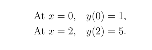
邊界條件

由于

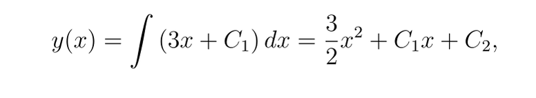
對 x 積分一次可得

再次積分,我們得到
現在,應用邊界條件:
-
對于 y(0)=1

-
對于 y(2)=5:
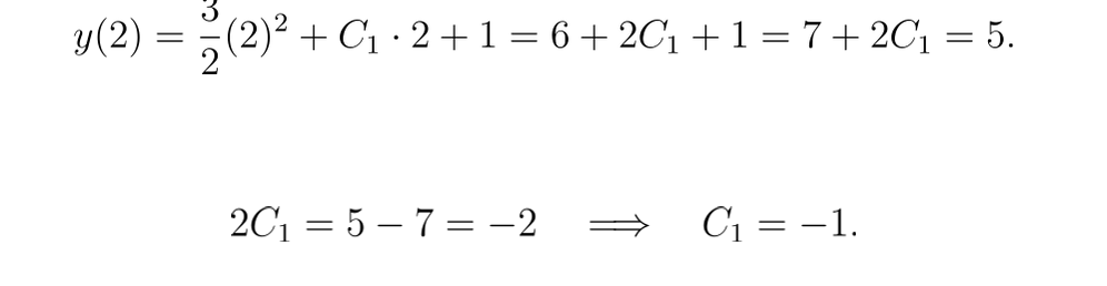
因此,解析解為:

用神經網絡解決微分方程
該方法稱為 PINN(物理信息神經網絡),在我們的示例中的工作方式如下:
神經網絡近似:
-
我們定義一個神經網絡 y(θ,x),其中 θ 表示網絡參數(權重和偏差)。該網絡旨在近似微分方程的解 y(x)。
-
在我們的例子中,神經網絡是一個小型全連接網絡(具有一個或多個隱藏層),它以空間坐標 x 作為輸入并輸出 y(x) 的近似值。
自動微分:
-
在這種情況下使用神經網絡的一個主要好處是大多數現代深度學習庫(如 PyTorch)都支持自動區分。
-
這意味著我們可以直接從網絡輸出計算關于輸入 x 的導數 y′(x) 和 y′′(x)。
殘差計算:
-
對于 ODE

我們將殘差 r(x) 定義為:

在網絡近似精確的點處,殘差應該為零。
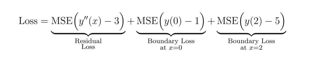
損失函數:
-
PINN 方法中的損失函數由兩部分組成:
-
殘差損失:在域內的一組內部搭配點處計算殘差 r(x) 的均方誤差 (MSE)。該項強制網絡的預測滿足微分方程。
-
邊界條件損失:網絡預測與給定邊界條件之間的差異的 MSE。
-
總損失為:
PINN的技術特性與創新點
PINN與傳統神經網絡的根本區別在于,它不依賴于標記數據集進行學習,而是將微分方程約束直接嵌入到損失函數中。這意味著模型學習得到的函數*yNN(x)*需同時滿足:
-
給定的微分方程約束條件
-
特定的邊界條件和初始條件
PINN框架中的偏微分方程(PDE)通常表示為:
![]()
其中

以二階微分方程為例:

這表明所求函數y(x)必須嚴格滿足該方程。
基于PINN求解微分方程的實踐案例
步驟1:?導入必要的庫函數
import?torch
import?torch.nn?as?nn
import?torch.optim?as?optim
import?matplotlib.pyplot?as?plt
import?numpy?as?np
步驟2:?定義 y(x) 的神經網絡近似值
class?ODE_Net(nn.Module):def?__init__(self, hidden_units=20):super(ODE_Net, self).__init__()self.layer1 = nn.Linear(1, hidden_units)self.layer2 = nn.Linear(hidden_units, hidden_units)self.layer3 = nn.Linear(hidden_units,?1)self.activation = nn.Tanh()def?forward(self, x):out = self.activation(self.layer1(x))out = self.activation(self.layer2(out))out = self.layer3(out)return?out
步驟3:計算 ODE 殘差
def?residual(model, x):"""Compute the ODE residual:y''(x) - 3 = 0."""# Enable gradients for xx.requires_grad_(True)y = model(x)# Compute first derivative: y'(x)dydx = torch.autograd.grad(y, x,grad_outputs=torch.ones_like(y),create_graph=True)[0]# Compute second derivative: y''(x)d2ydx2 = torch.autograd.grad(dydx, x,grad_outputs=torch.ones_like(dydx),create_graph=True)[0]# Compute the residual of the ODE: y''(x) - 3res = d2ydx2 -?3.0return?res
步驟4:損失函數
def?boundary_loss(model):"""Compute the loss associated with the boundary conditions:y(0)=1 and y(2)=5."""# Boundary condition at x=0: y(0)=1x0 = torch.tensor([[0.0]], device=device, requires_grad=True)y0 = model(x0)loss_bc0 = (y0 -?1.0)**2# Boundary condition at x=2: y(2)=5x2 = torch.tensor([[2.0]], device=device, requires_grad=True)y2 = model(x2)loss_bc2 = (y2 -?5.0)**2return?loss_bc0 + loss_bc2
步驟5:模型訓練
??# Initialize the model and optimizermodel = ODE_Net(hidden_units=20).to(device)optimizer = optim.Adam(model.parameters(), lr=1e-3)num_epochs =?5000# Generate interior points in the domain [0,2]N_interior =?50x_interior =?2?* torch.rand(N_interior,?1, device=device) ?# uniformly distributed in [0,2]# Training loop
for?epoch?in?range(num_epochs):model.train()optimizer.zero_grad()# Compute the residual loss at interior pointsr_interior = residual(model, x_interior)loss_res = torch.mean(r_interior**2)# Compute the boundary condition lossloss_bc = boundary_loss(model)# Total loss is the sum of the residual and boundary lossesloss = loss_res + loss_bcloss.backward()optimizer.step()if?epoch %?500?==?0:print(f"Epoch?{epoch}, Loss:?{loss.item():.6e}")# Evaluate and compare the solutionmodel.eval()x_test = torch.linspace(0,?2,?100, device=device).unsqueeze(1)y_pred = model(x_test).detach().cpu().numpy().flatten()x_test_np = x_test.cpu().numpy().flatten()
Epoch 0, Loss: 3.222174e+01
Epoch 500, Loss: 1.378794e-01
Epoch 1000, Loss: 5.264541e-03
Epoch 1500, Loss: 3.903809e-03
Epoch 2000, Loss: 3.040434e-03
Epoch 2500, Loss: 2.319159e-03
Epoch 3000, Loss: 1.656389e-03
Epoch 3500, Loss: 9.695904e-04
Epoch 4000, Loss: 4.545122e-04
Epoch 4500, Loss: 2.485181e-04
步驟6:對比精確度
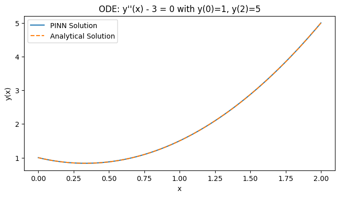
??# Analytical solution: y(x) = (3/2)x^2 - x + 1y_true =?1.5?* x_test_np**2?- x_test_np +?1plt.figure(figsize=(8,?4))plt.plot(x_test_np, y_pred, label="PINN Solution")plt.plot(x_test_np, y_true,?'--', label="Analytical Solution")plt.xlabel("x")plt.ylabel("y(x)")plt.legend()plt.title("ODE: y''(x) - 3 = 0 with y(0)=1, y(2)=5")plt.show()
使用 PINN 求解更復雜的 ODE
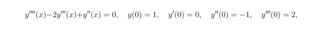
class?ODE_Net(nn.Module):def?__init__(self, hidden_units=20):super(ODE_Net, self).__init__()self.layer1 = nn.Linear(1, hidden_units)self.layer2 = nn.Linear(hidden_units, hidden_units)self.layer3 = nn.Linear(hidden_units, hidden_units)self.layer4 = nn.Linear(hidden_units,?1)self.activation = nn.Tanh()def?forward(self, x):out = self.activation(self.layer1(x))out = self.activation(self.layer2(out))out = self.activation(self.layer3(out))out = self.layer4(out)return?outdef?residual(model, x):x.requires_grad_(True)y = model(x)y_x = torch.autograd.grad(y, x, grad_outputs=torch.ones_like(y),create_graph=True)[0]y_xx = torch.autograd.grad(y_x, x, grad_outputs=torch.ones_like(y_x),create_graph=True)[0]y_xxx = torch.autograd.grad(y_xx, x, grad_outputs=torch.ones_like(y_xx),create_graph=True)[0]y_xxxx = torch.autograd.grad(y_xxx, x, grad_outputs=torch.ones_like(y_xxx),create_graph=True)[0] ? ?res = y_xxxx -?2*y_xxx + y_xxreturn?resdef?boundary_loss(model):x0 = torch.tensor([[0.0]], device=device, requires_grad=True)y0 = model(x0)y0_x = torch.autograd.grad(y0, x0, grad_outputs=torch.ones_like(y0),create_graph=True)[0]y0_xx = torch.autograd.grad(y0_x, x0, grad_outputs=torch.ones_like(y0_x),create_graph=True)[0]y0_xxx = torch.autograd.grad(y0_xx, x0, grad_outputs=torch.ones_like(y0_xx),create_graph=True)[0]bc1 = y0 -?1.0? ? ??# y(0) = 1bc2 = y0_x -?0.0? ??# y'(0) = 0bc3 = y0_xx - (-1.0) ?# y''(0) = -1 ?-> y0_xx + 1 = 0bc4 = y0_xxx -?2.0# y'''(0) = 2loss_bc = bc1**2?+ bc2**2?+ bc3**2?+ bc4**2return?loss_bcdef?main():model = ODE_Net(hidden_units=20).to(device)optimizer = optim.Adam(model.parameters(), lr=1e-3)num_epochs =?10000N_interior =?50x_interior = torch.rand(N_interior,?1, device=device)for?epoch?in?range(num_epochs):model.train()optimizer.zero_grad()r_interior = residual(model, x_interior)loss_res = torch.mean(r_interior**2)loss_bc = boundary_loss(model) ? ? ? ?loss = loss_res + loss_bcloss.backward()optimizer.step()if?epoch %?500?==?0:print(f"Epoch?{epoch}, Loss:?{loss.item():.6e}")model.eval()x_test = torch.linspace(0,?1,?100, device=device).unsqueeze(1)y_pred = model(x_test).detach().cpu().numpy().flatten()x_test_np = x_test.cpu().numpy().flatten()# Analytical solution: y(x) = 8 + 4x - 7e^x + 3xe^xy_true =?8?+?4*x_test_np -?7*np.exp(x_test_np) +?3*x_test_np*np.exp(x_test_np)plt.figure(figsize=(8,4))plt.plot(x_test_np, y_pred, label="Solution using PINN")plt.plot(x_test_np, y_true,?'--', label="Analytical solution")plt.xlabel("x")plt.ylabel("y(x)")plt.legend()plt.show()if?__name__ ==?"__main__":main()
Epoch 0, Loss: 6.779857e+00
Epoch 500, Loss: 2.092192e-01
Epoch 1000, Loss: 4.828146e-02
Epoch 1500, Loss: 3.233620e-02
Epoch 2000, Loss: 3.518355e-04
Epoch 2500, Loss: 2.392017e-04
Epoch 3000, Loss: 1.745588e-04
Epoch 3500, Loss: 1.332138e-04
Epoch 4000, Loss: 1.039377e-04
Epoch 4500, Loss: 3.754102e-03
Epoch 5000, Loss: 7.414911e-05
Epoch 5500, Loss: 5.272599e-05
Epoch 6000, Loss: 4.189969e-05
Epoch 6500, Loss: 1.759992e-03
Epoch 7000, Loss: 1.593289e-04
Epoch 7500, Loss: 2.400937e-05
Epoch 8000, Loss: 8.885263e-03
Epoch 8500, Loss: 6.434955e-05
Epoch 9000, Loss: 1.761451e-05
Epoch 9500, Loss: 1.477061e-05
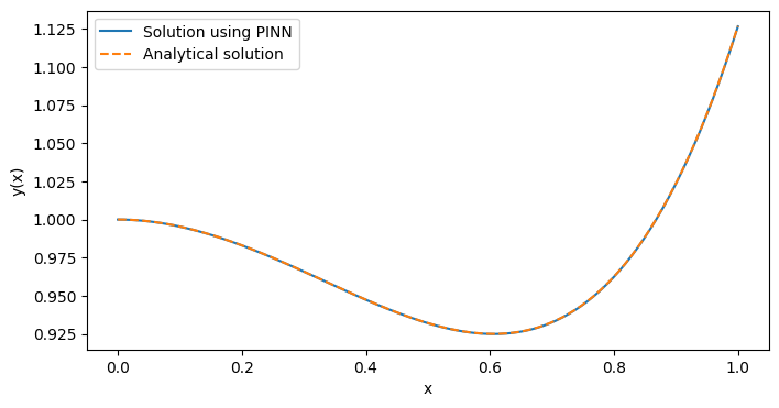
通過結果可以看出,我們已經成功地使用PINN方法求解了上述微分方程,并獲得了與解析解高度一致的數值解。
寫在最后
物理信息神經網絡(PINN)代表了一種在微分方程求解領域的重要技術突破,它將深度學習與物理定律有機結合,為傳統數值求解方法提供了一種高效、數據驅動的替代方案。PINN方法不僅在理論上具有創新性,同時在實際應用中展現出廣闊的應用前景,為復雜物理系統的建模與分析提供了新的研究路徑。
:廣告創意審核的關鍵要點與實踐應用)


算法復習總結2——分治算法)

)

(只在真機上有用,模擬器會分開彈 ))
![[Godot] C#人物移動抖動解決方案](http://pic.xiahunao.cn/[Godot] C#人物移動抖動解決方案)


)

