曲線生成 | 圖解Dubins曲線生成原理(附ROS C++/Python/Matlab仿真)

0 專欄介紹

🔥附C++/Python/Matlab全套代碼🔥課程設計、畢業設計、創新競賽必備！詳細介紹全局規劃(圖搜索、采樣法、智能算法等)；局部規劃(DWA、APF等)；曲線優化(貝塞爾曲線、B樣條曲線等)。

🚀詳情：圖解自動駕駛中的運動規劃(Motion Planning)，附幾十種規劃算法

1 什么是Dubins曲線？

Dubins曲線是指由美國數學家 Lester Dubins 在20世紀50年代提出的一種特殊類型的最短路徑曲線。這種曲線通常用于描述在給定轉彎半徑下的無人機、汽車或船只等載具的最短路徑，其特點是起始點和終點處的切線方向和曲率都是已知的。

在這里插入圖片描述

Dubins曲線包括直線段和最大轉彎半徑下的圓弧組成，通過合適的組合可以實現從一個姿態到另一個姿態的最短路徑規劃。這種曲線在航空、航海、自動駕駛等領域具有廣泛的應用，能夠有效地規劃航行路徑，減少能量消耗并提高效率。

2 Dubins曲線原理

2.1 坐標變換

如圖所示，在全局坐標系 $x O y$ 中，設機器人起始位姿、終止位姿、最小轉彎半徑分別為 $\left( x_s,y_s,\alpha \right)$ 、 $\left( x_g,y_g,\beta \right)$ 與 $R$ ，則以 $\boldsymbol{p}_s=\left( x_s,y_s \right)$ 為新坐標系原點， $\boldsymbol{p}_s$ 指向 $\boldsymbol{p}_g=\left( x_g,y_g \right)$ 方向為 $x^{'}$ 軸，垂直方向為 $y^{'}$ 軸建立新坐標系 $x^{'} O^{'} y^{'}$ 。

在這里插入圖片描述

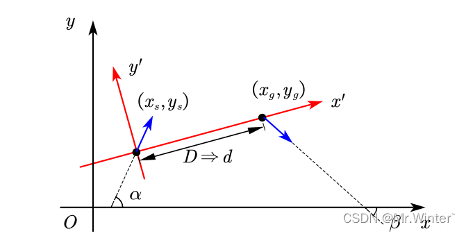
根據比例關系 ${{d}/{D}}={{r}/{R}}$ ，其中 $D=\left\| \boldsymbol{p}_s-\boldsymbol{p}_g \right\| _2$ 。為了便于后續推導，不妨歸一化最小轉彎半徑，即令 $r = 1$ 。所以在坐標系 $x^{'} O^{'} y^{'}$ 中，通常取起點、終點間距為 $d={{D}/{R}}$ ，從而起始位姿、終止位姿、最小轉彎半徑分別轉換為

$\mathrm{start}=\left[ \begin{matrix} 0& 0& \alpha -\theta\\\end{matrix} \right] ^T, \mathrm{goal}=\left[ \begin{matrix} d& 0& \beta -\theta\\\end{matrix} \right] ^T, r=1$

其中 $\theta =\mathrm{arc}\tan \left( {{\left( y_g-y_s \right)}/{\left( x_g-x_s \right)}} \right)$ ，接下來的推導均基于轉換坐標系 $x^{'} O^{'} y^{'}$ 。

2.2 單步運動公式

對于直行運動，設沿直線行進距離為 $l$ ，則

$\left[ \begin{matrix} x^*& y^*& \phi ^*\\\end{matrix} \right] ^T=\left[ \begin{matrix} x+l\cos \phi& y+l\sin \phi& \phi\\\end{matrix} \right] ^T$

對于轉彎運動，假設轉向角為 $\psi$ ，則由弧長公式可得

$l=\psi r\xlongequal{r=1}\psi$

因此設沿圓弧行進距離為 $l$ ，以左轉為例，由幾何關系易得

$\left[ \begin{matrix} x^*& y^*& \phi ^*\\\end{matrix} \right] ^T=\left[ \begin{matrix} x+r\sin \left( \phi +\psi \right) -r\sin \left( \phi \right)& y+r\cos \left( \phi +\psi \right) +r\cos \left( \phi \right)& \phi +\psi\\\end{matrix} \right] ^T$

代入 $r = 1$ 、 $\psi=l$ 可得

$\left[ \begin{matrix} x^*& y^*& \phi ^*\\\end{matrix} \right] ^T=\left[ \begin{matrix} x+\sin \left( \phi +l \right) -\sin \left( \phi \right)& y+\cos \left( \phi +l \right) +\cos \left( \phi \right)& \phi +l\\\end{matrix} \right] ^T$

同理，對于右轉而言，有

$\left[ \begin{matrix} x^*& y^*& \phi ^*\\\end{matrix} \right] ^T=\left[ \begin{matrix} x-\sin \left( \phi -l \right) +\sin \left( \phi \right)& y+\cos \left( \phi +l \right) -\cos \left( \phi \right)& \phi -l\\\end{matrix} \right] ^T$

綜上所述，可得單步運動映射

$\begin{cases} L_{l}^{+}\left( x,y,\phi \right) =\left[ \begin{matrix} x+\sin \left( \phi +l \right) -\sin \left( \phi \right)& y-\cos \left( \phi +l \right) +\cos \left( \phi \right)& \phi +l\\\end{matrix} \right] ^T\\ R_{l}^{+}\left( x,y,\phi \right) =\left[ \begin{matrix} x-\sin \left( \phi -l \right) +\sin \left( \phi \right)& y+\cos \left( \phi -l \right) -\cos \left( \phi \right)& \phi -l\\\end{matrix} \right] ^T\\ S_{l}^{+}\left( x,y,\phi \right) =\left[ \begin{matrix} x+l\cos \phi& y+l\sin \phi& \phi\\\end{matrix} \right] ^T\\\end{cases}$

2.3 曲線模式

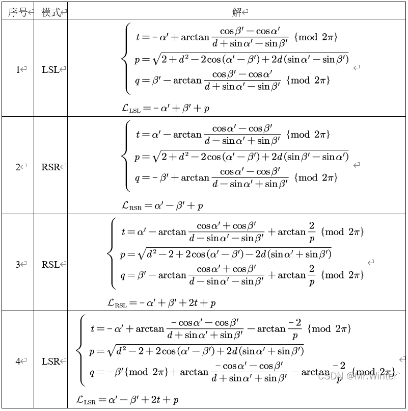
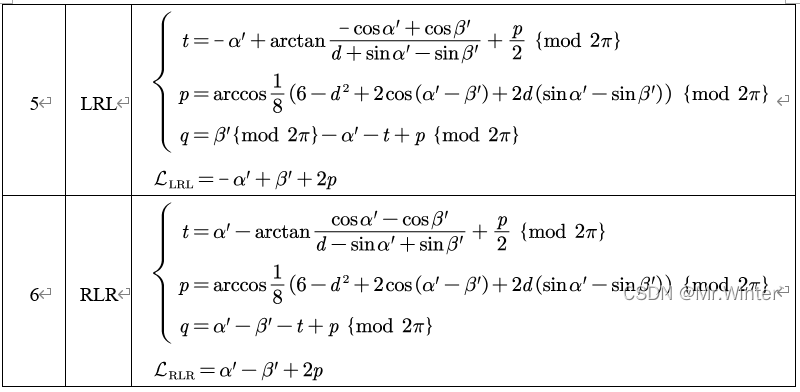
Dubins曲線假設物體只能向前，通過組合左轉、右轉、直行可得六種運動模式

$\left\{ LSL, RSR, RSL, LSR, RLR, LRL \right\}$

可以總結這六種運動模式的解析解為

在這里插入圖片描述

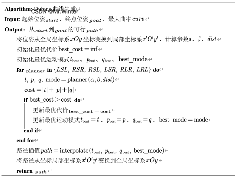
3 Dubins曲線生成算法

Dubins曲線路徑生成算法流程如表所示

在這里插入圖片描述

4 仿真實現

4.1 ROS C++實現

核心代碼如下所示

Points2d Dubins::generation(Pose2d start, Pose2d goal)
{Points2d path;double sx, sy, syaw;double gx, gy, gyaw;std::tie(sx, sy, syaw) = start;std::tie(gx, gy, gyaw) = goal;// coordinate transformationgx -= sx;gy -= sy;double theta = helper::mod2pi(atan2(gy, gx));double dist = hypot(gx, gy) * max_curv_;double alpha = helper::mod2pi(syaw - theta);double beta = helper::mod2pi(gyaw - theta);// select the best motionDubinsMode best_mode;double best_cost = DUBINS_MAX;DubinsLength length;DubinsLength best_length = { DUBINS_NONE, DUBINS_NONE, DUBINS_NONE };DubinsMode mode;for (const auto solver : dubins_solvers){(this->*solver)(alpha, beta, dist, length, mode);_update(length, mode, best_length, best_mode, best_cost);}if (best_cost == DUBINS_MAX)return path;// interpolation...// coordinate transformationEigen::AngleAxisd r_vec(theta, Eigen::Vector3d(0, 0, 1));Eigen::Matrix3d R = r_vec.toRotationMatrix();Eigen::MatrixXd P = Eigen::MatrixXd::Ones(3, path_x.size());for (size_t i = 0; i < path_x.size(); i++){P(0, i) = path_x[i];P(1, i) = path_y[i];}P = R * P;for (size_t i = 0; i < path_x.size(); i++)path.push_back({ P(0, i) + sx, P(1, i) + sy });return path;
}

4.2 Python實現

核心代碼如下所示

def generation(self, start_pose: tuple, goal_pose: tuple):sx, sy, syaw = start_posegx, gy, gyaw = goal_pose# coordinate transformationgx, gy = gx - sx, gy - sytheta = self.mod2pi(math.atan2(gy, gx))dist = math.hypot(gx, gy) * self.max_curvalpha = self.mod2pi(syaw - theta)beta = self.mod2pi(gyaw - theta)# select the best motionplanners = [self.LSL, self.RSR, self.LSR, self.RSL, self.RLR, self.LRL]best_t, best_p, best_q, best_mode, best_cost = None, None, None, None, float("inf")for planner in planners:t, p, q, mode = planner(alpha, beta, dist)if t is None:continuecost = (abs(t) + abs(p) + abs(q))if best_cost > cost:best_t, best_p, best_q, best_mode, best_cost = t, p, q, mode, cost# interpolation...# coordinate transformationrot = Rot.from_euler('z', theta).as_matrix()[0:2, 0:2]converted_xy = rot @ np.stack([x_list, y_list])x_list = converted_xy[0, :] + sxy_list = converted_xy[1, :] + syyaw_list = [self.pi2pi(i_yaw + theta) for i_yaw in yaw_list]return best_cost, best_mode, x_list, y_list, yaw_list

在這里插入圖片描述

4.3 Matlab實現

核心代碼如下所示

function [x_list, y_list, yaw_list] = generation(start_pose, goal_pose, param)sx = start_pose(1); sy = start_pose(2); syaw = start_pose(3);gx = goal_pose(1); gy = goal_pose(2); gyaw = goal_pose(3);% coordinate transformationgx = gx - sx; gy = gy - sy;theta = mod2pi(atan2(gy, gx));dist = hypot(gx, gy) * param.max_curv;alpha = mod2pi(syaw - theta);beta = mod2pi(gyaw - theta);% select the best motionplanners = ["LSL", "RSR", "LSR", "RSL", "RLR", "LRL"];best_cost = inf;best_segs = [];best_mode = [];for i=1:length(planners)planner = str2func(planners(i));[segs, mode] = planner(alpha, beta, dist);if isempty(segs)continueendcost = (abs(segs(1)) + abs(segs(2)) + abs(segs(3)));if best_cost > costbest_segs = segs;best_mode = mode;best_cost = cost;endend% interpolation...% coordinate transformationrot = [cos(theta), -sin(theta); sin(theta), cos(theta)];converted_xy = rot * [x_list; y_list];x_list = converted_xy(1, :) + sx;y_list = converted_xy(2, :) + sy;for j=1:length(yaw_list)yaw_list(j) = pi2pi(yaw_list(j) + theta);end
end