卷積神經網絡實現藝術風格化

基于卷積神經網絡實現圖片風格的遷移，可以用于大學生畢業設計基于python，深度學習，tensorflow卷積神經網絡， 通過Vgg16實現，一幅圖片內容特征的基礎上添加另一幅圖片的風格特征從而生成一幅新的圖片。在卷積模型訓練中，通過輸入固定的圖片來調整網絡的參數從而達到利用圖片訓練網絡的目的。而在生成特定風格圖片時，固定已有的網絡參數不變，調整圖片從而使圖片向目標風格轉化。在內容風格轉換時，調整圖像的像素值，使其向目標圖片在卷積網絡輸出的內容特征靠攏。在風格特征計算時，通過多個神經元的輸出兩兩之間作內積求和得到Gram矩陣，然后對G矩陣做差求均值得到風格的損失函數。

示例代碼：

import time
import numpy as np
import tensorflow as tf
from PIL import Image
from keras import backend
from keras.models import Model
from keras.applications.vgg16 import VGG16
from scipy.optimize import fmin_l_bfgs_b
from scipy.misc import imsave 

加載和預處理內容和樣式圖像

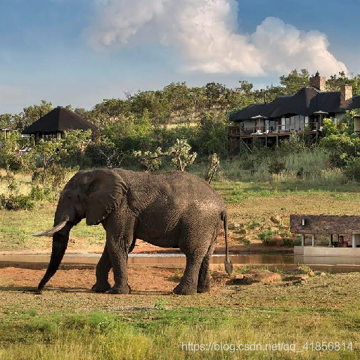
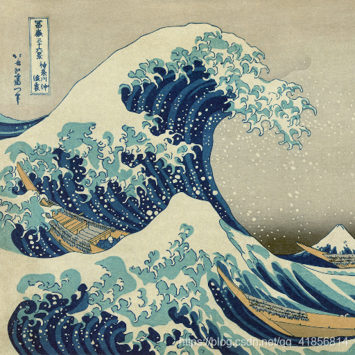
加載內容和樣式圖像，注意，我們正在處理的內容圖像質量不是特別高，但是在這個過程結束時我們將得到的輸出看起來仍然非常好。

height = 512
width = 512
content_image_path = 'images/elephant.jpg'
content_image = Image.open(content_image_path)
content_image = content_image.resize((height, width))
content_image

style_image_path = 'images/styles/wave.jpg'
style_image = Image.open(style_image_path)
style_image = style_image.resize((height, width))
style_image

然后，我們將這些圖像轉換成適合于數值處理的形式。
特別注意，我們添加了另一個維度（高度x寬度x 3維度）

以便我們可以稍后將這兩個圖像的表示連接到一個公共數據結構中。

content_array = np.asarray(content_image, dtype='float32')
content_array = np.expand_dims(content_array, axis=0)
print(content_array.shape)style_array = np.asarray(style_image, dtype='float32')
style_array = np.expand_dims(style_array, axis=0)
print(style_array.shape)

(1, 512, 512, 3)
(1, 512, 512, 3)

我們需要執行兩個轉換：

1.從每個像素中減去平均RGB值 (具體原因可查論文此處原因暫時省略)

2.將多維數組的順序從RGB翻轉到BGR（本文中使用的順序）。

content_array[:, :, :, 0] -= 103.939
content_array[:, :, :, 1] -= 116.779
content_array[:, :, :, 2] -= 123.68
content_array = content_array[:, :, :, ::-1]style_array[:, :, :, 0] -= 103.939
style_array[:, :, :, 1] -= 116.779
style_array[:, :, :, 2] -= 123.68
style_array = style_array[:, :, :, ::-1]

現在我們可以使用這些數組在Keras的后端（TensorFlow圖）中定義變量了。
我們還引入了一個占位符變量來存儲組合圖像，
該圖像在合并樣式圖像的樣式時保留了內容圖像的內容。

content_image = backend.variable(content_array)
style_image = backend.variable(style_array)
combination_image = backend.placeholder((1, height, width, 3))

NOISE_RATIO = 0.6
def generate_noise_image(content_image, noise_ratio = NOISE_RATIO):"""Returns a noise image intermixed with the content image at a certain ratio."""noise_image = np.random.uniform(-20, 20,(1, height, width, 3)).astype('float32')# White noise image from the content representation. Take a weighted average# of the valuesinput_image = noise_image * noise_ratio + content_image * (1 - noise_ratio)return input_image

content_image = tf.Variable(content_array,dtype=tf.float32)style_image = tf.Variable(style_array,dtype=tf.float32)# combination_image = tf.placeholder(dtype=tf.float32,shape = (1,height,width,3))combination_image = tf.Variable(initial_value=generate_noise_image(content_image))

最后，我們將所有這些圖像數據連接到一個張量中，
該張量適合用Keras’VGG16模型進行處理。

input_tensor = backend.concatenate([content_image,style_image,combination_image], axis=0) #作用 將兩個變量和占位符數據集成
input_tensor = tf.concat([content_image,style_image,combination_image],axis = 0)
input_tensor

重新使用預先訓練的圖像分類模型來定義損失函數

由于我們對分類問題不感興趣，因此不需要完全連接的層或最終的softmax分類器。我們只需要下表中用綠色標記的那部分型號。

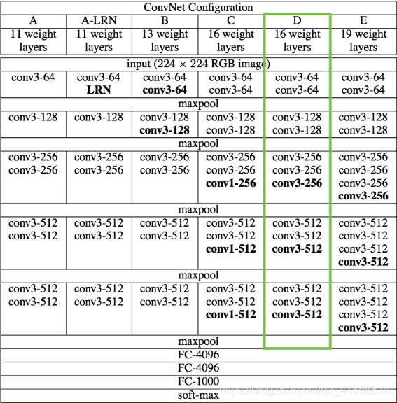
對于我們來說，訪問這個被截斷的模型是很簡單的，因為Keras附帶了一組預先訓練的模型，包括我們感興趣的VGG16模型。注意，通過在下面的代碼中設置“include_top=False”，我們不包括任何完全連接的層。

model = VGG16(input_tensor=input_tensor, weights='imagenet',include_top=False)

<keras.engine.training.Model at 0x267f261f208>

從上表可以看出，我們使用的模型有很多層。對于這些層，Keras有自己的名稱。讓我們列出這些名稱，以便以后可以方便地引用各個層。

layers = dict([(layer.name, layer.output) for layer in model.layers])
layers

讀取本地模型

import scipy as scipydef load_vgg_model(path):"""Returns a model for the purpose of 'painting' the picture.Takes only the convolution layer weights and wrap using the TensorFlowConv2d, Relu and AveragePooling layer. VGG actually uses maxpool butthe paper indicates that using AveragePooling yields better results.The last few fully connected layers are not used.Here is the detailed configuration of the VGG model:0 is conv1_1 (3, 3, 3, 64)1 is relu2 is conv1_2 (3, 3, 64, 64)3 is relu    4 is maxpool5 is conv2_1 (3, 3, 64, 128)6 is relu7 is conv2_2 (3, 3, 128, 128)8 is relu9 is maxpool10 is conv3_1 (3, 3, 128, 256)11 is relu12 is conv3_2 (3, 3, 256, 256)13 is relu14 is conv3_3 (3, 3, 256, 256)15 is relu16 is maxpool17 is conv4_1 (3, 3, 256, 512)18 is relu19 is conv4_2 (3, 3, 512, 512)20 is relu21 is conv4_3 (3, 3, 512, 512)22 is relu23 is maxpool24 is conv5_1 (3, 3, 512, 512)25 is relu26 is conv5_2 (3, 3, 512, 512)27 is relu28 is conv5_3 (3, 3, 512, 512)29 is relu30 is maxpool31 is fullyconnected (7, 7, 512, 4096)32 is relu33 is fullyconnected (1, 1, 4096, 4096)34 is relu35 is fullyconnected (1, 1, 4096, 1000)36 is softmax"""vgg = scipy.io.loadmat(path)vgg_layers = vgg['layers']def _weights(layer, expected_layer_name):"""Return the weights and bias from the VGG model for a given layer.layers[0][0][0][0][2][0][0]"""W = vgg_layers[0][layer][0][0][2][0][0]b = vgg_layers[0][layer][0][0][2][0][1]layer_name = vgg_layers[0][layer][0][0][0]assert layer_name == expected_layer_namereturn W, bdef _relu(conv2d_layer):"""Return the RELU function wrapped over a TensorFlow layer. Expects aConv2d layer input."""return tf.nn.relu(conv2d_layer)def _conv2d(prev_layer, layer, layer_name):"""Return the Conv2D layer using the weights, biases from the VGGmodel at 'layer'."""W, b = _weights(layer, layer_name)W = tf.constant(W)b = tf.constant(np.reshape(b, (b.size)))return tf.nn.conv2d(prev_layer, filter=W, strides=[1, 1, 1, 1], padding='SAME') + bdef _conv2d_relu(prev_layer, layer, layer_name):"""Return the Conv2D + RELU layer using the weights, biases from the VGGmodel at 'layer'."""return _relu(_conv2d(prev_layer, layer, layer_name))#     def _avgpool(prev_layer):
#         """
#         Return the AveragePooling layer.#         return tf.nn.avg_pool(prev_layer, ksize=[1, 2, 2, 1], strides=[1, 2, 2, 1], padding='SAME')def _avgpool(prev_layer):return tf.nn.max_pool(prev_layer,ksize=[1,2,2,1],strides=[1,2,2,1],padding='SAME')# Constructs the graph model.graph = {}graph['input']   = input_tensorgraph['conv1_1']  = _conv2d_relu(graph['input'], 0, 'conv1_1')graph['conv1_2']  = _conv2d_relu(graph['conv1_1'], 2, 'conv1_2')graph['_maxpool1'] = _avgpool(graph['conv1_2'])graph['conv2_1']  = _conv2d_relu(graph['_maxpool1'], 5, 'conv2_1')graph['conv2_2']  = _conv2d_relu(graph['conv2_1'], 7, 'conv2_2')graph['_maxpool2'] = _avgpool(graph['conv2_2'])graph['conv3_1']  = _conv2d_relu(graph['_maxpool2'], 10, 'conv3_1')graph['conv3_2']  = _conv2d_relu(graph['conv3_1'], 12, 'conv3_2')graph['conv3_3']  = _conv2d_relu(graph['conv3_2'], 14, 'conv3_3')graph['_maxpool3'] = _avgpool(graph['conv3_3'])graph['conv4_1']  = _conv2d_relu(graph['_maxpool3'], 17, 'conv4_1')graph['conv4_2']  = _conv2d_relu(graph['conv4_1'], 19, 'conv4_2')graph['conv4_3']  = _conv2d_relu(graph['conv4_2'], 21, 'conv4_3')graph['_maxpool4'] = _avgpool(graph['conv4_3'])graph['conv5_1']  = _conv2d_relu(graph['_maxpool4'], 24, 'conv5_1')graph['conv5_2']  = _conv2d_relu(graph['conv5_1'], 26, 'conv5_2')graph['conv5_3']  = _conv2d_relu(graph['conv5_2'], 28, 'conv5_3')graph['_maxpool5'] = _avgpool(graph['conv5_3'])return graph

from scipy import io
import tensorflow as tf
model = load_vgg_model('./imagenet-vgg-verydeep-16.mat')

如果你盯著上面的單子看，你會相信我們已經把所有我們想要的東西都放在桌子上了（綠色的單元格）。還要注意，因為我們為Keras提供了一個具體的輸入張量，所以各種張量流張量得到了定義良好的形狀。

---

風格轉換問題可以作為一個優化問題

其中我們希望最小化的損失函數可以分解為三個不同的部分：內容損失、風格損失和總變化損失。

這些項的相對重要性由一組標量權重決定。這些都是任意的，但是在經過相當多的實驗之后選擇了下面的集合，以找到一個生成對我來說美觀的輸出的集合。

content_weight = 0.025
style_weight = 5.0
total_variation_weight = 1.0

我們現在將使用模型的特定層提供的特征空間來定義這三個損失函數。我們首先將總損失初始化為0，然后分階段將其相加。

loss = tf.Variable(0.)
loss

content_loss

content_loss 是內容的特征表示與組合圖像之間的（縮放，平方）歐氏距離。

def content_loss(content, combination):return tf.reduce_sum(tf.square(combination - content))layer_features = model['conv2_2']
content_image_features = layer_features[0, :, :, :]
combination_features = layer_features[2, :, :, :]loss += content_weight * content_loss(content_image_features,combination_features)

風格損失

這就是事情開始變得有點復雜的地方。

對于樣式丟失，我們首先定義一個稱為Gram matrix的東西。該矩陣的項與對應特征集的協方差成正比，從而捕獲關于哪些特征傾向于一起激活的信息。通過只捕獲圖像中的這些聚合統計信息，它們對圖像中對象的特定排列是盲目的。這使他們能夠捕獲與內容無關的樣式信息。（這根本不是微不足道的，我指的是[試圖解釋這個想法的論文] 。

通過對特征空間進行適當的重構并取外積，可以有效地計算出Gram矩陣。

def gram_matrix(x):features = backend.batch_flatten(backend.permute_dimensions(x, (2, 0, 1)))gram = backend.dot(features, backend.transpose(features))return gram

#也可用tf的方法 不使用kears的后端
# def gram_matrix(x):
#     ret = tf.transpose(x, (2, 0, 1))
#     features = tf.reshape(ret,[ret.shape[0],-1])
#     gram = tf.matmul(features,tf.transpose(features))
#     return gram

樣式損失是樣式和組合圖像的Gram矩陣之間的差的（縮放，平方）Frobenius范數。

同樣，在下面的代碼中，我選擇使用Johnson等人定義的圖層中的樣式特性。（2016）而不是蓋蒂等人。（2015）因為我覺得最終的結果更美觀。我鼓勵你嘗試這些選擇，以看到不同的結果。

def style_loss(style, combination):S = gram_matrix(style)C = gram_matrix(combination)channels = 3size = height * widthreturn tf.reduce_sum(tf.square(S - C)) / (4. * (channels ** 2) * (size ** 2))feature_layers = ['conv1_2', 'conv2_2','conv3_3', 'conv4_3','conv5_3']
for layer_name in feature_layers:layer_features = model[layer_name]style_features = layer_features[1, :, :, :]combination_features = layer_features[2, :, :, :]sl = style_loss(style_features, combination_features)loss += (style_weight / len(feature_layers)) * sl

總變化損失

現在我們回到了更簡單的基礎上。

如果您只使用我們目前介紹的兩個損失項（樣式和內容）來解決優化問題，您會發現輸出非常嘈雜。因此，我們增加了另一個術語，稱為[總變化損失]（一個正則化項），它鼓勵空間平滑。

您可以嘗試減少“總變化”權重，并播放生成圖像的噪聲級別。

combination_image

def total_variation_loss(x):a = tf.square(x[:, :height-1, :width-1, :] - x[:, 1:, :width-1, :])b = tf.square(x[:, :height-1, :width-1, :] - x[:, :height-1, 1:, :])return tf.reduce_sum(tf.pow(a + b, 1.25))loss += total_variation_weight * total_variation_loss(combination_image) 
optimizer = tf.train.AdamOptimizer(0.001).minimize(loss)
optimizer

定義所需的梯度并解決優化問題

現在，我們已經對輸入圖像進行了處理，并定義了了損失函數 calculators，
剩下的工作就是定義相對于組合圖像的總損失的梯度，
并使用這些梯度對組合圖像進行迭代改進，以最小化損失。

grads = backend.gradients(loss, combination_image)
grads

然后，我們需要定義一個“Evaluator”類，
它通過兩個單獨的函數“loss”和“grads”檢索丟失和漸變。

之所以這樣做，是因為“scipy.optimize”需要單獨的函數來處理損失和梯度，但是單獨計算它們將是低效的。

outputs = [loss]
outputs += grads
f_outputs = backend.function([combination_image], outputs)def eval_loss_and_grads(x):x = x.reshape((1, height, width, 3))outs = f_outputs([x])loss_value = outs[0]grad_values = outs[1].flatten().astype('float64')return loss_value, grad_valuesclass Evaluator(object):def __init__(self):self.loss_value = Noneself.grads_values = Nonedef loss(self, x):assert self.loss_value is Noneloss_value, grad_values = eval_loss_and_grads(x)self.loss_value = loss_valueself.grad_values = grad_valuesreturn self.loss_valuedef grads(self, x):assert self.loss_value is not Nonegrad_values = np.copy(self.grad_values)self.loss_value = Noneself.grad_values = Nonereturn grad_valuesevaluator = Evaluator()

現在我們終于可以解決我們的優化問題了。這個組合圖像的生命開始于一個隨機的（有效的）像素集合，我們使用[L-BFGS]算法（一個比標準梯度下降更快收斂的準牛頓算法）迭代改進它。

我在2次迭代之后就停止了，因為時間問題，可以定義十次左右，效果較好損失可以自己觀察。

evaluator.grads

x = np.random.uniform(0, 255, (1, height, width, 3)) - 128.iterations = 2for i in range(iterations):print('Start of iteration', i)start_time = time.time()x, min_val, info = fmin_l_bfgs_b(evaluator.loss, x.flatten(),fprime=evaluator.grads, maxfun=20)print('Current loss value:', min_val)end_time = time.time()print('Iteration %d completed in %ds' % (i, end_time - start_time))

Start of iteration 0
Current loss value: 73757336000.0
Iteration 0 completed in 217s
Start of iteration 1
Current loss value: 36524343000.0
Iteration 1 completed in 196s

效果圖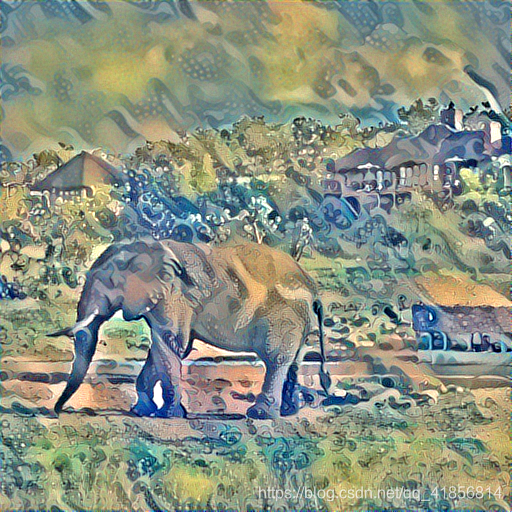

總結

盡管這段代碼的輸出非常漂亮，但用來生成它的過程非常緩慢。
不管你如何加速這個算法（使用gpu和創造性的黑客），
它仍然是一個相對昂貴的問題來解決。
這是因為我們每次想要生成圖像時都在解決一個完整的優化問題。

---

PS：公眾號內回復 ：Python，即可獲取最新最全學習資源！

    破解專業版pycharm參考博客www.wakemeupnow.cn公眾號：劉旺學長

內容詳細：【個人分享】今年最新最全的Python學習資料匯總！！！

以上，便是今天的分享，希望大家喜歡，
覺得內容不錯的，歡迎點擊分享支持，謝謝各位。

單純分享，無任何利益相關！