Many of us have heard, read, or even performed an A/B Test before, which means we have conducted a statistical test at some point. Most of the time, we have worked with data from first or third-party sources and performed these tests with ease by either using tools ranging from Excel to Statistical Software and even more automated solutions such as Google Optimize.

我們當中許多人以前都聽過，讀過甚至進行過A / B測試，這意味著我們在某個時候進行了統計測試。 在大多數情況下，我們使用第一方或第三方來源的數據，并使用Excel到Statistics Software等工具以及更自動化的解決方案(例如Google Optimize)輕松地執行了這些測試。

If you are like me, you might be curious about how these types of tests work and how concepts such as Type I and Type II Error, Confidence Intervals, Effect Magnitude, Statistical Power, and others interact with each other.

如果您像我一樣，可能會對這些類型的測試如何工作以及類型I和類型II錯誤 ， 置信區間 ， 影響幅度 ， 統計 功效以及其他概念之間的交互方式感到好奇。

In this post, I would like to invite you to take a different approach for one specific type of A/B test, which makes use of a particular statistic called Chi-Squared. In particular, I will try to explore and walk through this type of test by taking the great but long road of simulations, avoiding libraries and tables, hopefully managing to explore and build some of the intuition behind it.

在本文中，我想邀請您對一種特定類型的A / B測試采用不同的方法，該方法利用稱為Chi-Squared的特定統計量。 特別是，我將嘗試通過漫長而漫長的模擬之路，避免使用庫和表，希望設法探索并建立其背后的一些直覺 ，從而探索并完成此類測試。

開始之前 (Before we start)

Even though we could use data from our past experiments or even third-party sources such as Kaggle, it would be more convenient for this post to generate our data. It will allow us to compare our conclusions with a known ground truth; otherwise, it will be most likely unknown.

即使我們可以使用過去實驗中的數據，甚至可以使用第三方來源(例如Kaggle)中的數據，對于本帖子來說，生成我們的數據也會更加方便。 它可以使我們將結論與已知的事實相比較; 否則，很可能未知。

For this example, we will generate a dummy dataset that will represent six different versions of a signup form and the number of leads we observed on each. For this dummy set to be random and have a winner version that will serve us as ground truth, we will generate this table by simulating some biased dice’s throws.

對于此示例，我們將生成一個虛擬數據集，該數據集將表示六個不同版本的注冊表單以及我們在每個表單上觀察到的潛在客戶數量。 為了使這個虛擬集是隨機的，并且有一個獲勝者版本將用作 基礎事實，我們將通過模擬一些有偏向的骰子投擲來生成此表。

For this, we have generated an R function that simulates a biased dice in which we have a 20% probability of lading in 6 while a 16% chance of landing in any other number.

為此，我們生成了一個R函數，該函數模擬了一個有偏見的骰子，在該骰子中，我們有20％的概率在6中提貨，而在其他數字中有16％的機會著陸。

# Biased Dice Rolling Function
DiceRolling <- function(N) {
    Dices <- data.frame()
    for (i in 1:6) {
      if(i==6) {
        Observed <- data.frame(Version=as.character(LETTERS[i]),Signup=rbinom(N/6,1,0.2))
      } else {
        Observed <- data.frame(Version=as.character(LETTERS[i]),Signup=rbinom(N/6,1,0.16))
      }
      Dices <- rbind(Dices,Observed)
    }
    return(Dices)
}# Let's roll some dices
set.seed(123) # this is for result replication 86
Dices <- DiceRolling(1800)

Think of each Dice number as a representation of a different landing version (1–6 or A-F). For each version, we will throw our Dice 300 times, and we will write down its results as follows:

將每個骰子編號視為不同著陸版本(1-6或AF)的表示。 對于每個版本，我們將擲骰子300次，并將其結果記錄如下：

• If we are on version A (1) and throw the Dice and it lands on 1, we consider it to be Signup; otherwise, just a visit.
  如果我們使用版本A(1)并將骰子扔到1，則認為它是Signup； 否則，只是一次訪問。
• We repeat 300 times for each version.
  每個版本重復300次。

樣本數據 (Sample Data)

As commented earlier, this is what we got:

如前所述，這是我們得到的：

# We shuffle our results
set.seed(25) 
rows <- sample(nrow(Dices))
t(Dices[head(rows,10),])

We can observe from our first ten results that we got one Signup for F, D, and A. In aggregated terms, our table looks like this:

我們可以從前十個結果中觀察到，我們為F ， D和A獲得了一個Signup 。總的來說，我們的表如下所示：

library(ggplot2)
ggplot(Result, aes(x=Version, y=Signup)) + geom_bar(stat="identity", position="dodge") + ggtitle("Summary Chart")
Result <- aggregate(Signup ~ Version, Dices, sum)
t(Result)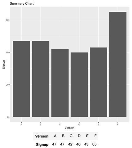

From now own, think of this table as Dice throws, eCommerce conversions, surveys, or a Landing Page Signup Conversion as we will use here, it does not matter, use whatever is more intuitive for you.

從現在開始，將此表視為Dice投擲，電子商務轉換，調查或著陸頁注冊轉換，就像我們將在此處使用的那樣，這沒關系，可以使用對您而言更直觀的方式。

For us, it will be signups, so we should produce this report:

對于我們來說，這將是注冊，因此我們應該生成此報告：

觀察頻率 (Observed Frequencies)

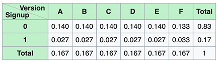
We will now aggregate our results, including both our Signup (1) and Did not Signup (0) results, which will allow us to understand better how these differ from our expected values or frequencies; this is also called a Cross Tabulation or Contingency Table.

現在，我們將匯總我們的結果，包括“ 注冊”(1)和“未注冊”(0)結果，這將使我們能夠更好地了解這些結果與預期值或頻率之間的差異； 這也稱為交叉表或列聯表 。

# We generate our contigency table
Observed <- table(Dices)
t(Observed)

In summary:

綜上所述：

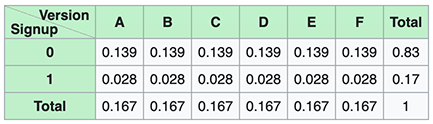
預期頻率 (Expected Frequencies)

Since we know how our Cross Tabulation looks, we can now generate a table simulating how we should expect our results to be like considering the same performance of all versions. It is equivalent to say that each version had the same Signup Conversion or probability in the case of our example or the expected result of a non-biased dice if you prefer.

由于我們知道交叉制表的外觀，因此我們現在可以生成一個表，該表模擬我們如何期望我們的結果像考慮所有版本的相同性能一樣。 可以說，在我們的示例中，每個版本都有相同的注冊轉換或概率，或者，如果您愿意，可以使用無偏向骰子的預期結果。

# We generate our expected frequencies table
Expected <- Observed
Expected[,1] <- (sum(Observed[,1])/nrow(Observed))
Expected[,2] <- sum(Observed[,2])/nrow(Observed)
t(Expected)

In summary:

綜上所述：

假設檢驗 (Hypothesis Testing)

We know our test had a higher-performing version not only by visually inspecting the results but because we purposely designed it to be that way.

我們知道我們的測試具有更高性能的版本，不僅是通過目視檢查結果，還因為我們有目的地將其設計為這種方式。

This is the moment we have waited for: is it possible for us to prove this solely based on the results we got?.

這是我們等待的時刻： 是否有可能僅根據獲得的結果來證明這一點？ 。

The answer is yes, and the first step is to define our Null and Alternative Hypothesis, which we will later try to accept or reject.

答案是肯定的，第一步是定義零假設和替代假設，我們稍后將嘗試接受或拒絕。

Our alternative hypothesis (H1) is what we want to prove correct, which states that there is, in fact, a relationship between the landing version and the result we observed. In contrast, our null hypothesis states that there is no relationship meaning there is no significant difference between our observed and expected frequencies.

我們要證明的另一種假設(H1)是正確的，它指出著陸版本與我們觀察到的結果之間實際上存在某種關系。 相反，我們的零假設指出沒有關系，這意味著我們的觀測頻率與預期頻率之間沒有顯著差異。

統計 (Statistic)

Our goal is to find how often our observed data is located in a universe where our null hypothesis is correct, meaning, where our observed and expected signup frequencies have no significant difference.

我們的目標是找到我們的觀測數據位于原假設正確的宇宙中的頻率，即我們的觀測和預期簽約頻率無顯著差異。

A useful statistic that’s able to sum up all these values; six columns (one for each version) and two rows (one for each signup state) into a single value is Chi-Square, which is calculated as follows:

有用的統計信息，能夠匯總所有這些值； 六個值(每個版本一個)和兩行(每個注冊狀態一個)組成一個值是Chi-Square，其計算方式如下：

We will not get into details of how this formula can be found neither of its assumptions or requirements (such as Yates Correction), because it is not the subject of this post. On the contrary, we would like to perform a numerical approach through simulations, which should shed some light on these types of hypothesis tests.

我們不會詳細介紹如何從公式的任何假設或要求(例如Yates Correction)中都找不到該公式，因為它不是本文的主題。 相反，我們想通過仿真執行數值方法，這應該為這些類型的假設檢驗提供一些啟發。

Resuming, if we compute this formula with our data, we get:

繼續，如果我們使用我們的數據計算此公式，則會得到：

# We calculate our X^2 score
Chi <- sum((Expected-Observed)^2/Expected)
Chi

空分布模擬 (Null Distribution Simulation)

We need to obtain the probability of finding a statistic as extreme as the one we observed, which in this case, is represented by Chi-Square equal to 10.368. This, in terms of probability, is also known as our P-Value.

我們需要獲得找到與我們觀察到的統計數據一樣極端的統計數據的概率，在本例中，該統計數據由卡方表示為10.368。 就概率而言，這也稱為我們的P值 。

For this, we will simulate a Null Distribution as a benchmark. What this means is that we need to generate a scenario in which our Null Distribution is correct, suggesting a situation where there is no relationship between the landing version and the observed signup results (frequencies) we got.

為此，我們將模擬空分布作為基準。 這意味著我們需要生成一個空分布正確的方案，這表明著陸版本與我們觀察到的注冊結果(頻率)之間沒有關系 。

A solution that rapidly comes to mind is to repeat our experiment from scratch, either by re-collecting results many times or, as in the context of this post, using an unbiased dice to compare how our observed results behave in contrast to these tests. Even though this might seem intuitive at first, in real-world scenarios, this solution might not be the most efficient one since it would require extreme use of resources such as time and budget to repeat this A/B test many times.

Swift想到的解決方案是從頭開始重復我們的實驗，方法是多次重新收集結果，或者如本文所述，使用無偏小骰子來比較觀察到的結果與這些測試相比的表現。 盡管起初看起來似乎很直觀，但在實際情況下，此解決方案可能并不是最有效的解決方案，因為它需要大量使用資源(例如時間和預算)才能多次重復進行此A / B測試。

重采樣 (Resampling)

An excellent solution to the problem discussed above is called resampling. What resampling does is make one variable independent of the other by shuffling one of them randomly. If there were an initial relationship between them, this relation would be lost due to the random sampling method.

解決上述問題的一種極好的解決方案稱為重采樣。 重采樣的作用是通過隨機地對其中一個變量進行改組，使一個變量與另一個變量無關。 如果它們之間存在初始關系，則由于隨機抽樣方法，該關系將丟失。

In particular, we need to use the original (unaggregated) samples for this scenario. We will later permutate one of the columns several times, which will be Signup status in this case.

特別是，在這種情況下，我們需要使用原始(未匯總)樣本。 稍后，我們將對其中一列進行多次排列，在本例中為“注冊”狀態。

In particular, let us see an example of 2 shuffles for the first “10 samples” shown earlier:

特別是，讓我們看一下前面顯示的第一個“ 10個樣本”的2個隨機播放的示例：

Let us try it now with the complete (1800) sample set:

現在讓我們嘗試使用完整的樣本集(1800)：

Permutation #1

排列＃1

Perm1 <- Dices
set.seed(45)
Perm1$Signup <- sample(Dices$Signup)
ResultPerm1 <- aggregate(Signup ~ Version, Perm1, sum)
cat("Permutation #1:\n\n")
cat("Summary\n\n")
t(ResultPerm1)
cat("Chi-Squared")
Perm1Observed <- table(Perm1)
sum((Expected-Perm1Observed)^2/Expected)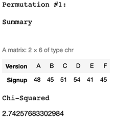

Permutation #2

排列＃2

Perm1 <- Dices
set.seed(22)
Perm1$Signup <- sample(Dices$Signup)
ResultPerm1 <- aggregate(Signup ~ Version, Perm1, sum)
cat("Permutation #2:\n\n")
cat("Summary\n\n")
t(ResultPerm1)
cat("Chi-Squared")
Perm1Observed <- table(Perm1)
sum((Expected-Perm1Observed)^2/Expected)

As seen in both permutations of our data, we got utterly different summaries and Chi-Squared values. We will repeat this process a bunch of times to explore what we can obtain at a massive scale.

從我們的數據的兩個排列中可以看出，我們得到了完全不同的匯總和Chi-Squared值。 我們將重復此過程很多次，以探索我們可以大規模獲得的東西。

模擬 (Simulation)

Let us simulate 15k permutations of our data.

讓我們模擬數據的15k排列。

# Simulation Function
Simulation <- function(Dices,k) {
    dice_perm <- data.frame()
    i <- 0
    while(i < k) {
      i <- i + 1;# We permutate our Results
      permutation$Signup <- sample(Dices$Signup)# We generate our contigency table
      ObservedPerm <- table(permutation)# We generate our expected frequencies table
      ExpectedPerm <- ObservedPerm
      ExpectedPerm[,1] <- (sum(ObservedPerm[,1])/nrow(ObservedPerm))
      ExpectedPerm[,2] <- sum(ObservedPerm[,2])/nrow(ObservedPerm)# We calculate X^2 test for our permutation
      ChiPerm <- sum((ExpectedPerm-ObservedPerm)^2/ExpectedPerm)# We add our test value to a new dataframe
      dice_perm <- rbind(dice_perm,data.frame(Permutation=i,ChiSq=ChiPerm))
    }
return(dice_perm)
}# Lest's resample our data 15.000 times
start_time <- Sys.time()
permutation <- Dicesset.seed(12)
permutation <- Simulation(Dices,15000)
end_time <- Sys.time()
end_time - start_time

重采樣分布 (Resample Distribution)

As we can observe below, our 15k permutations look like it is distributed with a distinct shape and resembles, as expected, a Chi-Square distribution. With this information, we can now calculate how many of the 15k iterations, we observed a Chi-Squared value as extreme as our initial 10.36 calculation.

正如我們在下面可以看到的，我們的15k排列看起來像是分布有不同的形狀，并且與預期的卡方分布相似。 有了這些信息，我們現在可以計算出15k迭代中有多少次，我們觀察到的Chi-Squared值與我們最初的10.36計算一樣極端。

totals <- as.data.frame(table(permutation$ChiSq))
totals$Var1 <- as.numeric(as.character(totals$Var1))
plot( totals$Freq ~ totals$Var1, ylab=”Frequency”, xlab=”Chi-Squared Values”,main=”Null Distribution”)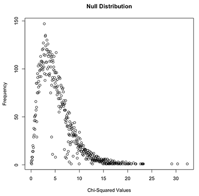

P值 (P-Value)

Let us calculate how many times we obtained a Chi-Square value equal to or higher than 10.368 (our calculated score).

讓我們計算獲得等于或高于10.368(我們的計算得分)的卡方值的次數。

Higher <- nrow(permutation[which(permutation$ChiSq >= Chi),])
Total <- nrow(permutation)
prob <- Higher/Total
cat(paste("Total Number of Permutations:",Total,"\n"))
cat(paste("  - Total Number of Chi-Squared Values equal to or higher than",round(Chi,2),":",Higher,"\n"))
cat(paste("  - Percentage of times it was equal to or higher (",Higher,"/",Total,"): ",round(prob*100,3),"% (P-Value)",sep=""))

決策極限 (Decision Limits)

We now have our P-Value, which means that if the Null Hypothesis is correct, saying there is no relationship between Version and Signups, we should encounter a Chi-Square as extreme only a small 6.5% of the time. If we think of this as only dice results, we should expect “results as biased as ours” even by throwing an unbias dice at most 6.5% of the time.

現在，我們有了P值，這意味著如果零假設是正確的，也就是說版本和注冊之間沒有關系，那么我們應該僅在很小的6.5％的時間內遇到卡方。 如果我們認為這只是骰子的結果，那么即使最多最多擲6.5％的時間來獲得無偏見的骰子，我們也應該期望“結果像我們一樣有偏見”。

Now we need to define our decision limits on which we accept or reject our null hypothesis.

現在，我們需要定義我們接受或拒絕原假設的決策極限。

We calculated our decision limits for 90%, 95%, and 99% confidence intervals, meaning which Chi-Squared values we should expect as a limit on those odds.

我們計算了90％，95％和99％置信區間的決策極限，這意味著我們應該期望將Chi-Squared值作為這些幾率的極限。

# Decition Limits
totals <- as.data.frame(table(permutation$ChiSq))
totals$Var1 <- as.numeric(as.character(totals$Var1))
totals$Prob <- cumsum(totals$Freq)/sum(totals$Freq)
Interval90 <- totals$Var1[min(which(totals$Prob >= 0.90))]
Interval95 <- totals$Var1[min(which(totals$Prob >= 0.95))]
Interval975 <- totals$Var1[min(which(totals$Prob >= 0.975))]
Interval99 <- totals$Var1[min(which(totals$Prob >= 0.99))]cat(paste("Chi-Squared Limit for 90%:",round(Interval90,2),"\n"))
cat(paste("Chi-Squared Limit for 95%:",round(Interval95,2),"\n"))
cat(paste("Chi-Squared Limit for 99%:",round(Interval99,2),"\n"))

Fact Check

事實檢查

As observed by the classical “Chi-Square Distribution Table”, we can find very similar values from the ones we obtained from our simulation, which means our confidence intervals and P-Values should be very accurate.

正如經典“卡方分布表”所觀察到的，我們可以從模擬中獲得非常相似的值，這意味著我們的置信區間和P值應該非常準確。

假設檢驗 (Hypothesis Testing)

As we expected, we can reject the Null Hypothesis and claim that there is a significant relationship between versions and signups. Still, there is a small caveat, and this is our level of confidence. As observed in the calculations above, we can see that our P-Value (6.5%) is just between 90% and 95% confidence intervals, which means, even though we can reject our Null Hypothesis with 90% confidence, we cannot reject it at 95% or any superior confidence level.

如我們所料，我們可以拒絕零假設，并聲稱版本和注冊之間存在重要關系。 仍然有一點需要注意，這就是我們的信心水平 。 從上面的計算中可以看出，我們可以看到P值(6.5％)介于90％和95％的置信區間之間，這意味著，即使我們可以90％的置信度拒絕零假設，我們也不能拒絕它95％或更高的置信度。

If we claim to have 90% confidence, then we are also claiming there is a 10% chance of wrongly rejecting our null hypothesis (also called Type I Error, False Positive, or Alpha). Note, in reality, such standard arbitrary values (90%,95%, 99%) are used, but we could easily claim we are 93.5% certain since we calculated a 6.5% probability of a Type I Error.

如果我們聲稱擁有90％的置信度，那么我們還聲稱有10％的機會錯誤地拒絕了我們的零假設(也稱為I型錯誤 ， 誤報或Alpha )。 注意，實際上，使用了此類標準任意值(90％，95％，99％)，但由于我們計算出I型錯誤的概率為6.5％ ，因此我們可以很容易地斷言我們具有93.5％的確定性。

Interestingly, even though we know for sure there is a relationship between version and signups, we cannot prove this by mere observation, simulations, and neither by doing this hypothesis test with a standard 95% confidence level. This concept of failing to reject our Null Hypothesis even though we know it is wrong is called a false negative or Type II Error (Beta), which is dependent on the Statistical Power of this test, which measures the probability that this does not happen.

有趣的是，即使我們確定知道版本和注冊之間存在關聯，我們也不能僅僅通過觀察，模擬以及通過以標準的95％置信度進行假設檢驗來證明這一點。 即使我們知道錯誤假設也不會拒絕零假設的概念稱為假陰性或II型錯誤 ( Beta )，這取決于此測試的統計功效 ，該度量衡量了這種情況不會發生的可能性。

統計功效 (Statistical Power)

In our hypothesis test, we saw we were unable to reject our Null Hypothesis even at standard values intervals such as 95% confidence or more. This is due to the Statistical Power (or Power) of the test we randomly designed, which is particularly sensitive to our statistical significance criterion discussed above (alpha or Type I error) and both effect magnitude and sample sizes.

在我們的假設檢驗中，我們看到即使在標準值間隔(例如95％置信度或更高)下也無法拒絕零假設。 這是由于我們隨機設計的測試的統計 功效 (或功效 )，這對我們上面討論的統計顯著性標準(alpha或I型誤差)以及影響幅度和樣本量特別敏感。

Power is calculated as follows:

功率計算如下：

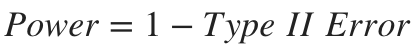
In particular, we can calculate our current statistical Power by answering the following question:

特別是，我們可以通過回答以下問題來計算當前的統計功效：

• If we were to repeat our experiment X amount of times and calculate our P-Value on each experiment, which percent of the times, we should expect a P-Value as extreme as 5%?
  如果我們要重復實驗X次并在每個實驗中計算出我們的P值(占百分比的百分比)，那么我們應該期望P值達到5％的極限嗎？

Let us try answering this question:

讓我們嘗試回答這個問題：

MultipleDiceRolling <- function(k,N) {
    pValues <- NULL
    for (i in 1:k) {
    Dices <- DiceRolling(N)    
    Observed <- table(Dices)
    pValues <- cbind(pValues,chisq.test(Observed)$p.value)
    i <- i +1
    }
    return(pValues)
}# Lets replicate our experiment (1800 throws of a biased dice) 10k times
start_time <- Sys.time()
Rolls <- MultipleDiceRolling(10000,1800)
end_time <- Sys.time()
end_time - start_time

How many times did we observe P-Values as extreme as 5%?

我們觀察過多少次P值高達5％？

cat(paste(length(which(Rolls <= 0.05)),"Times"))

Which percent of the times did we observe this scenario?

我們觀察到這種情況的百分比是多少？

Power <- length(which(Rolls <= 0.05))/length(Rolls)
cat(paste(round(Power*100,2),"% of the times (",length(which(Rolls <= 0.05)),"/",length(Rolls),")",sep=""))

As calculated above, we observe a Power equivalent to 21.91% (0.219), which is quite low since the gold standard is around 0.8 or even 0.9 (90%). In other words, this means we have a 78.09% (1 — Power) probability of making a Type II Error or, equivalently, a 78% chance of failing to reject our Null Hypothesis at a 95% confidence interval even though it is false, which is what happened here.

根據上面的計算，我們觀察到的功效等于21.91％(0.219)，這是非常低的，因為金標準約為0.8甚至0.9(90％)。 換句話說，這意味著我們有78.09％(1- Power)發生II型錯誤的概率，或者等效地， 即使它是假的 ， 也有78％的機會未能在95％的置信區間內拒絕零假設 ，這就是這里發生的事情。

As mentioned, Power is a function of:

如前所述，Power是以下功能之一：

• Our significance criterion: this is our Type I Error or Alpha, which we decided to be 5% (95% confidence).

  我們的顯著性標準 ：這是我們的I類錯誤或Alpha，我們決定為5％(置信度為95％)。

• Effect Magnitude or Size: This represents the difference between our observed and expected values in terms of the standardized statistic of use. In this case, since we used Chi-Square statistic, this effect (named w) is calculated as the squared root of the normalized Chi-Square value and is usually categorized as Small (0.1), Medium (0.3), and Large (0.5) (Ref: Cohen, J. (1988).)

  影響幅度或大小 ：這表示我們的觀察值與期望值之間的差異(使用標準化的使用統計數據)。 在這種情況下，由于我們使用的是卡方統計量，因此將此效果(稱為w )計算為歸一化卡方值的平方根，通常分為小(0.1)，中(0.3)和大(0.5)。 )(參考資料： Cohen，J.(1988)。 )

• Sample size: This represents the total amount of samples (in our case, 1800).

  樣本數量 ：代表樣本總數(在我們的示例中為1800)。

效果幅度 (Effect Magnitude)

We designed an experiment with a relatively small effect magnitude since our Dice was only biased in one face (6) with only a slight additional chance of landing in its favor.

我們設計的實驗的效果等級相對較小，因為我們的骰子僅偏向一張臉(6)，只有很少的其他機會落在其臉上。

In simple words, our effect magnitude (w) is calculated as follows:

簡而言之，我們的影響幅度(w)計算如下：

1) Where our Observed Proportions are calculated as follow:

1)我們的觀察比例計算如下：

Probabilities of our alternative hypothesis

我們的替代假設的概率

2) And our Expected Proportions:

2)和我們的預期比例 ：

Probabilities of our null hypothesis

原假設的概率

Finally, we can obtain our effect size as follows:

最后，我們可以獲得如下效果大小：

樣本量 (Sample Size)

Similarly to our effect size, our sample sizes, even though it seems of enough magnitude (1800), is not big enough to spot relationship (or bias) at 95% confidence since our effect size, as we calculated, was very small. We can expect an inverse relationship between sample sizes and effect magnitude. The more significant the effect, the lower the sample size needed to prove it at a given significance level.

與我們的效應量相似，我們的樣本量即使看起來足夠大(1800)，也不足以在95％的置信度上發現關系(或偏差)，因為我們計算出的效應量很小。 我們可以預期樣本量與效應量之間存在反比關系。 效果越顯著，在給定的顯著性水平下證明該結果所需的樣本量越少。

At this time, it might be more comfortable to think sample sizes of our A/B test as dice or even coin throws. It is somewhat intuitive that with one dice/coin throw, we will be unable to spot a biased dice/coin, but if 1800 throws are not high enough to detect this small effect at a 95% confidence level, this leads us to the following question: how many throws do we need?

目前，將A / B測試的樣本大小視為擲骰子甚至投擲硬幣可能會更舒服。 從一個直觀的角度來看，擲一枚骰子/硬幣，我們將無法發現有偏見的骰子/硬幣，但是如果1800枚硬幣的高度不足以在95％的置信度水平上檢測到這種小影響，這將導致我們得出以下結論：問題：我們需要多少次擲球？

The same principle applies to the sample size of our A/B test. The lesser the effect, such as small variations in conversion from small changes in each version (colors, fonts, buttons), the bigger the sample and, therefore, the time we need to collect the data required to accept or reject our hypothesis. A common problem in many A/B tests concerning website conversion in eCommerce is that tools such as Google Optimize can take many days, if not weeks, and most of the time, we do not encounter a conclusive answer.

同樣的原則適用于我們的A / B測試的樣本量。 效果越小(例如，每個版本(顏色，字體，按鈕)的微小變化帶來的轉換變化很小)，樣本就越大，因此，我們需要收集接受或拒絕我們的假設所需的數據的時間也越大。 在許多與電子商務中的網站轉換有關的A / B測試中，一個普遍的問題是，諸如Google Optimize之類的工具可能要花費很多天(如果不是幾周的話)，并且在大多數情況下，我們沒有得到最終的答案。

To solve this, first, we need to define the Statistical Power we want. Next, we will try answering this question by iterating different values of N until we minimize the difference between our Expected Power and the Observed Power.

為了解決這個問題，首先，我們需要定義所需的統計功效。 接下來，我們將嘗試通過迭代N的不同值來回答這個問題，直到將期望功率和觀測功率之間的差異最小化為止。

# Basic example on how to obtain a given N based on a target Power.# Playing with initialization variables might be needed for different scenarios.
CostFunction <- function(n,w,p) {
  value <- pchisq(qchisq(0.05, df = 5, lower = FALSE), df = 5, ncp = (w^2)*n, lower = FALSE)
  Error <- (p-value)^2
  return(Error)
}
SampleSize <- function(w,n,p) {
    
    # Initialize variables
    N <- n
    i <- 0
    h <- 0.000000001
    LearningRate <- 40000000
    HardStop <- 20000
    power <- 0
    
    # Iteration loop
    for (i in 1:HardStop) {
      dNdError <- (CostFunction(N + h,w,p) - CostFunction(N,w,p)) / h
      N <- N - dNdError*LearningRate
      ChiLimit <- qchisq(0.05, df = 5, lower = FALSE)
      new_power <- pchisq(ChiLimit, df = 5, ncp = (w^2)*N, lower = FALSE)
      if(round(power,6) >= round(new_power,6)) {
        cat(paste0("Found in ",i," Iterations\n"))
        cat(paste0("   Power: ",round(power,2),"\n"))
        cat(paste0("   N: ",round(N)))
        break();
      }
      power <- new_power
      i <- i +1
    }
}
set.seed(22)
SampleSize(0.04,1800,0.8)
SampleSize(0.04,1800,0.9)

As seen above, after different iterations of N, we obtained a recommended sample of 8.017 and 10.293 for 0.8 and 0.9 Power values, respectively.

如上所示，在N的不同迭代之后，我們分別針對0.8和0.9的Power值獲得了推薦的樣本8.017和10.293。

Let us repeat the experiment from scratch and see which results we get for these new sample size of 8.017 suggested by aiming a commonly used Power of 0.8.

讓我們從頭開始重復該實驗，并查看針對這些新的8.017樣本大小(通過將常用功效設定為0.8)所獲得的結果。

start_time <- Sys.time()# Let's roll some dices
set.seed(11) # this is for result replication
Dices <- DiceRolling(8017) # We expect 80% Power
t(table(Dices))# We generate our contigency table
Observed <- table(Dices)# We generate our expected frequencies table
Expected <- Observed
Expected[,1] <- (sum(Observed[,1])/nrow(Observed))
Expected[,2] <- sum(Observed[,2])/nrow(Observed)# We calculate our X^2 score
Chi <- sum((Expected-Observed)^2/Expected)
cat("Chi-Square Score:",Chi,"\n\n")# Lest's resample our data 15.000 times
permutation <- Dices
set.seed(20)
permutation <- Simulation(Dices,15000)Higher <- nrow(permutation[which(permutation$ChiSq >= Chi),])
Total <- nrow(permutation)
prob <- Higher/Total
cat(paste("Total Number of Permutations:",Total,"\n"))
cat(paste("  - Total Number of Chi-Squared Values equal to or higher than",round(Chi,2),":",Higher,"\n"))
cat(paste("  - Percentage of times it was equal to or higher (",Higher,"/",Total,"): ",round(prob*100,3),"% (P-Value)\n\n",sep=""))# Lets replicate this new experiment (8017 throws of a biased dice) 20k times
set.seed(20)
Rolls <- MultipleDiceRolling(10000,8017)
Power <- length(which(Rolls <= 0.05))/length(Rolls)
cat(paste(round(Power*100,3),"% of the times (",length(which(Rolls <= 0.05)),"/",length(Rolls),")",sep=""))end_time <- Sys.time()
end_time - start_time

最后的想法 (Final Thoughts)

As expected by our new experiment design of sample size equal to 8017, we were able to reduce our P-Value to 1.9%.

正如我們新的樣本量等于8017的實驗設計所預期的那樣，我們能夠將P值降低到1.9％。

Additionally, we observe a Statistical Power equivalent to 0.79 (very near our goal), which implies we were able to reduce our Type II Error (non-rejection of our false null hypothesis) to just 21%!

此外，我們觀察到的統計功效等于0.79(非常接近我們的目標)，這意味著我們能夠將II型錯誤(不拒絕錯誤的虛假假設)降低到21％！

This allows us to conclude with 95% confidence (in reality 98.1%) that there is, as we always knew, a statistically significant relationship between Landing Version and Signups. Now we need to test, with a given confidence level, which version was the higher performer; this will be covered in a similar future post.

這使我們能夠以95％的信心(實際上是98.1％)得出結論，正如我們一直知道的那樣，著陸版本和注冊之間存在統計上顯著的關系。 現在我們需要在給定的置信度下測試哪個版本的性能更高； 這將在以后的類似文章中介紹。

If you have any questions or comments, do not hesitate to post them below.

如果您有任何問題或意見，請隨時在下面發布。