有關深層學習的FAU講義 (FAU LECTURE NOTES ON DEEP LEARNING)

These are the lecture notes for FAU’s YouTube Lecture “Deep Learning”. This is a full transcript of the lecture video & matching slides. We hope, you enjoy this as much as the videos. Of course, this transcript was created with deep learning techniques largely automatically and only minor manual modifications were performed. Try it yourself! If you spot mistakes, please let us know!

這些是FAU YouTube講座“ 深度學習 ”的 講義 。 這是演講視頻和匹配幻燈片的完整記錄。 我們希望您喜歡這些視頻。 當然，此成績單是使用深度學習技術自動創建的，并且僅進行了較小的手動修改。 自己嘗試！ 如果發現錯誤，請告訴我們！

導航 (Navigation)

Previous Lecture / Watch this Video / Top Level / Next Lecture

上一個講座 / 觀看此視頻 / 頂級 / 下一個講座

Welcome back to deep learning! So today, we want to look into the applications of known operator learning and a particular one that I want to show today is CT reconstruction.

歡迎回到深度學習！ 因此，今天，我們要研究已知的操作員學習的應用程序，而我今天要展示的特定應用是CT重建。

So here, you see the formal solution to the CT reconstruction problem. This is the so-called filtered back-projection or Radon inverse. This is exactly the equation that I referred to earlier that has already been solved in 1917. But as you may know, CT scanners have only been realized in 1971. So actually, Radon who found this very nice solution has never seen it put to practice. So, how did he solve the CT reconstruction problem? Well, CT reconstruction is a projection process. It’s essentially a linear system of equations that can be solved. The solution is essentially described by a convolution and a sum. So, it’s a convolution along the detector direction s and then a back-projection over the rotation angle θ. During the whole process, we suppress negative values. So, we kind of also get a non-linearity into the system. This all can also be expressed in matrix notation. So, we know that the projection operations can simply be described as a matrix A that describes how the rays intersect with the volume. With this matrix, you can simply take the volume x multiplied with A and this gives you the projections p that you observe in the scanner. Now, getting the reconstruction is you take the projections p and you essentially need some kind of inverse or pseudo-inverse of A in order to compute this. We can see that there is a solution that is very similar to what we’ve seen in the above continuous equation. So, we have essentially a pseudo-inverse here and that is A transpose times A A transpose inverted times p. Now, you could argue that the inverse that you see here in a is actually the filter. So, for this particular problem, we know that the inverse of A A transpose will form a convolution.

因此，在這里，您將看到CT重建問題的正式解決方案。 這就是所謂的濾波反投影或Radon逆。 這正是我之前提到的方程式，該方程式在1917年已經解決。但是，您可能知道，CT掃描儀直到1971年才實現。因此，實際上，發現這種非常好的解決方案的Radon從未見過將其付諸實踐。 。 那么，他是如何解決CT重建問題的呢？ 好吧，CT重建是一個投影過程。 從本質上講，這是一個可以求解的線性方程組。 該解決方案基本上由卷積和和來描述。 因此，它是沿著檢測器方向s的卷積，然后是旋轉角度θ上的反投影。 在整個過程中，我們抑制負值。 因此，我們也將非線性引入系統中。 所有這些也可以用矩陣符號表示。 因此，我們知道投影操作可以簡單地描述為矩陣A ，該矩陣A描述光線與體積的相交方式。 使用此矩陣，您只需將體積x乘以A，就可以得出在掃描儀中觀察到的投影p。 現在，要進行重構，您需要獲得投影p，并且您實際上需要某種A的逆或偽逆才能進行計算。 我們可以看到，有一個解決方案與上面的連續方程式非常相似。 因此，這里我們基本上有一個偽逆，即A轉置時間A A轉置反向時間p 。 現在，您可以爭辯說，您在a中看到的逆實際上是過濾器。 因此，對于這個特定問題，我們知道AA轉置的逆會形成卷積。

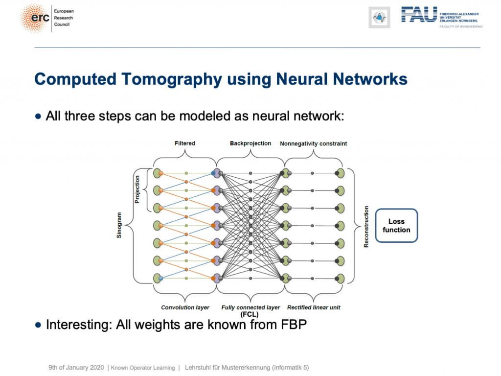
This is nice because we know how to implement convolutions into deep networks, right? Matrix multiplications! So, this is what we did. We can map everything into a neural network. We start on the left-hand side. We put in the Sinogram, i.e., all of the projections. We have a convolutional layer that is computing the filtered projections. Then, we have a back-projection that is a fully connected layer and it’s essentially this large matrix A. Finally, we have the non-negativity constraint. So essentially, we can define a neural network that does exactly filtered back-projection. Now, this is actually not so super interesting because there’s nothing to learn. We know all of those weights and by the way, the matrix A is really huge. For 3-D problems, it can approach up to 65,000 terabytes of memory in floating-point precision. So, you don’t want to instantiate this matrix. The reason why you don’t want to do that it that it’s very sparse. So, only a very small fraction of the elements in A are actual connections. This is very nice for CT reconstruction because then you typically never instantiate A but you compute A and A transpose simply using raytracers. This is typically done on a graphics board. Now, why are we talking about all of this? Well, we’ve seen there are cases where CT reconstruction is insufficient and we could essentially do trainable CT reconstruction.

很好，因為我們知道如何將卷積實現為深度網絡，對嗎？ 矩陣乘法！ 因此，這就是我們所做的。 我們可以將所有內容映射到神經網絡。 我們從左側開始。 我們輸入了Singram，即所有的預測。 我們有一個卷積層，用于計算濾波后的投影。 然后，我們有一個反投影，它是一個完全連接的層，本質上就是這個大矩陣A。 最后，我們有非負約束。 因此，從本質上講，我們可以定義一個精確過濾反向投影的神經網絡。 現在，這實際上并不是那么有趣，因為沒有什么可學的。 我們知道所有這些權重，順便說一下，矩陣A確實很大。 對于3D問題，它可以以浮點精度接近65,000 TB的內存。 因此，您不想實例化此矩陣。 您不想這樣做的原因是它非常稀疏。 因此， A中的元素中只有很小一部分是實際連接。 這對于CT重建非常好，因為您通常從不實例化A，而是僅使用光線跟蹤器計算A和A轉置。 這通常在圖形板上完成。 現在，我們為什么要談論所有這些？ 好吧，我們已經看到了CT重建不足的情況，并且我們基本上可以進行可訓練的CT重建。

Already, if you look at a CT book, you run into the first problems. If you implement it by the book and you just want to reconstruct a cylinder that is merely showing the value of one within this round area, then you would like to have an image like this one where everything is one within the cylinder and outside of the cylinder it’s zero. So, we’re showing this line plot here along the blue line through the original slice image. Now, if you just implement filtered back-projection, as you find it in the textbook, you get a reconstruction like this one. The typical mistake is that you choose the length of the Fourier transform too short and the other one is that you don’t consider the discretization appropriately. Now, you can work with this and fix the problem in the discretization. So what you can do now is essentially train the correct filter using learning techniques. So, what you would do in a classical CT class is you would run through all the math from the continuous integration to the discrete version in order to figure out the correct filter coefficients.

如果已經看了一本CT書，就會遇到第一個問題。 如果您通過書來實現它，而只想重建一個圓柱體，而該圓柱體僅顯示該圓形區域內一個圓柱體的值，那么您將希望獲得一個像這樣的圖像，其中一切都在圓柱體之內和之外。氣缸為零。 因此，我們在這里顯示此線圖，沿著原始切片圖像的藍線。 現在，如果您只是實現濾波后的反投影，就像在教科書中找到的那樣，您將獲得像這樣的重構。 一個典型的錯誤是您選擇傅立葉變換的長度太短，而另一個錯誤是您沒有適當考慮離散化。 現在，您可以使用它并解決離散化問題。 因此，您現在可以做的就是使用學習技術來訓練正確的濾波器。 因此，在經典的CT類中，您將經歷從連續積分到離散形式的所有數學運算，以便找出正確的濾波器系數。

Instead, here we show that by knowing that it takes the form of convolution, we can express our inverse simply as p times the Fourier transform which is also just a matrix multiplication F. Then, K is a diagonal matrix that holds the spectral weights followed an inverse Fourier transform that is denoted as F hermitian here. Lastly, you back-project. We can simply write this up as a set of matrices and by the way, this would then also define the network architecture. Now, we can actually optimize the correct filter weights. What we have to do is we have to solve the associate optimization problem. This is simply to have the right-hand side equal to the left-hand side and we choose an L2 loss.

取而代之的是，在這里我們表明，通過知道它采用卷積的形式，我們可以簡單地將逆表示為p乘傅里葉變換的p倍，這也是矩陣乘法F。 然后， K是一個對角矩陣，它保持頻譜權重，然后進行傅立葉逆變換，在此將其表示為F Hermitian。 最后，您進行背投影。 我們可以簡單地將其寫成一組矩陣，并且順便說一下，這也將定義網絡體系結構。 現在，我們實際上可以優化正確的過濾器權重。 我們需要做的是解決關聯優化問題。 這僅僅是使右手邊等于左手邊，我們選擇L2損失。

You’ve seen that on numerous occasions in this class. Now, if we do that, we can also compute this by hand. If you use the matrix cookbook then, you get the following gradient with respect to the layer K. This would be F times A times and then in brackets A transpose F hermitian our diagonal filter matrix K times the Fourier transform times p minus x and then times F times p transpose. So if you look at this, you can see that this is actually the reconstruction. This is the forward pass through our network. This is the error that is introduced. So, this is our sensitivity that we get at the end of the network if we apply our loss. We compute the sensitivity and then we backpropagate up to the layer where we actually need it. This is layer K. Then, we multiply with the activations that we have in this particular layer. If you remember our lecture on feed-forward networks, this is nothing else than the respective layer gradient. We still can reuse the math that we learned in this lecture very much earlier. So actually, we don’t have to go through the pain of computing this gradient. Our deep learning framework will do it for us. So, we can save a lot of time using the backpropagation algorithm.

您已經在本堂課中多次看到這一點。 現在，如果這樣做，我們也可以手動計算。 如果您使用矩陣食譜，則相對于K層，您將獲得以下漸變。 這將是F乘以A倍，然后在括號A中轉置F埃爾米特數，即我們的對角濾波器矩陣K乘以Fourier變換乘以p減去x ，再乘以F乘以p換位。 因此，如果您看一下，您可以看到這實際上是重構。 這是通過我們網絡的正向傳遞。 這是引入的錯誤。 因此，這是我們應用損失時在網絡末端獲得的敏感度。 我們計算靈敏度，然后反向傳播到實際需要它的層。 這是K層。 然后，我們乘以該特定層中的激活。 如果您還記得我們在前饋網絡上的演講 ，那無非就是各自的層梯度。 我們仍然可以重用很早之前在本堂課中學到的數學。 因此，實際上，我們不必經歷計算此梯度的麻煩。 我們的深度學習框架將為我們做到這一點。 因此，使用反向傳播算法可以節省大量時間。

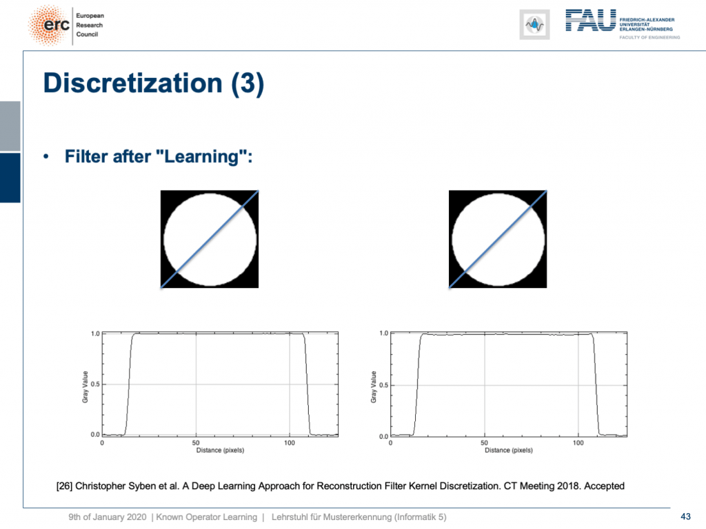
What happens if you do so? Well, of course, after learning the artifact is gone. So, you can remove this artifact. Well, this is kind of an academic example. We also have some more.

如果這樣做會怎樣？ 好吧，當然，在學習了神器之后就消失了。 因此，您可以刪除此工件。 好吧，這是一個學術例子。 我們還有更多。

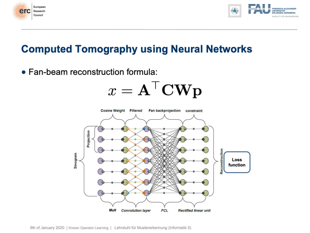
You can see that you can approximate also fan-beam reconstruction with similar matrix kinds of equations. We have now an additional matrix W. So, W is a point-wise weight that is multiplied to each pixel in the input image. C is now directly our convolutional matrix. So, we can describe a fan-beam reconstruction formula simply with this equation and of course, we can produce a resulting network out of this.

您會看到，您也可以使用類似矩陣類型的方程來近似扇形束重構。 現在，我們有一個附加矩陣W。 因此， W是逐點權重，它乘以輸入圖像中的每個像素。 C現在直接是我們的卷積矩陣。 因此，我們可以簡單地用該方程式來描述扇形束重建公式，當然，我們可以由此產生一個結果網絡。

Now let’s look at what happens if we go back to this limited angle tomography problem. So, if you have a complete scan, it looks like this. Let’s go to a scan that has only 180 degrees of rotation. Here, the minimal set for the scan would be actually 200 degrees. So, we are missing 20 degrees of rotation. Not as strong as the limited angle problem that I showed in the introduction of known operator learning, but still significant artifact emerges here. Now, let’s take as pre-training our traditional filtered back-projection algorithm and adjust the weights and the convolution. If you do so, you get this reconstruction. So, you can see that the image quality is dramatically improved. A lot of the artifact is gone. There are still some artifacts on the right-hand side, but image quality is dramatically better. Now, you could argue “Well, you are again using a black box!”.

現在讓我們看一下如果回到這個有限角度層析成像問題 。 因此，如果您有完整的掃描，則看起來像這樣。 讓我們轉到只有180度旋轉的掃描。 在這里，掃描的最小集實際上是200度。 因此，我們缺少20度旋轉。 雖然不如我在介紹已知的操作員學習中所介紹的有限角度問題那么強，但這里仍然出現了明顯的工件。 現在，讓我們對傳統的濾波反投影算法進行預訓練，并調整權重和卷積。 如果這樣做，您將獲得此重建。 因此，您可以看到圖像質量得到了顯著改善。 許多工件消失了。 右側仍然有一些偽像，但是圖像質量明顯更好。 現在，您可以爭論“嗯，您又在使用黑匣子！”。

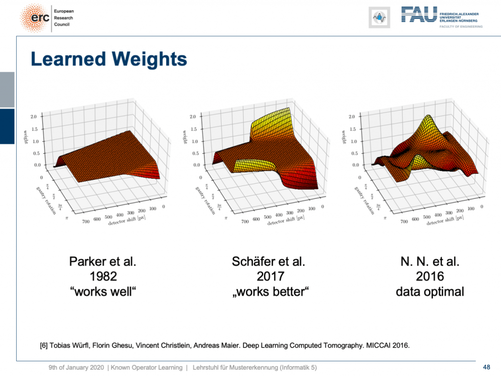
but that’s not actually true because our weights can be mapped back into the original interpretation. We still have a filtered back-projection algorithm. This means we can read out the trained weights from our network and compare them to the state-of-the-art. If you look here, we initialized with the so-called Parker weights which are the solution to a short scan. The idea here is that opposing rays are assigned a weight such that the rays that measure exactly the same line integrals essentially sum up to one. This is shown on the left-hand side. On the right-hand side, you find the solution that our neural network found in 2016. So this is the data-optimal solution. You see it did significant changes to our Parker weights. Now, in 2017 Sch?fer et al. published a heuristic how to fix these limited angle artifacts. They suggested ramping up the weight of rays that run through the area where we are missing observations. They simply increase the weight in order to fix the deterministic mass loss. What they found looks better, but is a heuristic. We can see that our neural network found a very similar solution and we can demonstrate that this is data-optimal. So, you can see a distinct difference on the very left and the very light right. If you look here and if you look here, you can see that in these weights, this goes all the way up here and here. This is actually the end of the detector. So, here and here is the boundary of the detector, also here and here. This means we didn’t have any change in these areas here and these areas here. The reason for that is we never had an object in the training data that would fill the entire detector. Hence, we can also not backpropagate gradients here. This is why we essentially have the original initialization still at these positions. That’s pretty cool. That’s really interpreting networks. That’s really understanding what’s happening in the training process, right?

但這并不是真的，因為我們的權重可以映射回原始解釋。 我們仍然有一個過濾的反投影算法。 這意味著我們可以從網絡中讀取經過訓練的權重，并將其與最新技術進行比較。 如果您在這里查看，我們將使用所謂的Parker權重進行初始化，這是短期掃描的解決方案。 這里的想法是為相對的光線分配權重，以使測量完全相同的線積分的光線本質上合計為一個。 這顯示在左側。 在右側，您可以找到我們的神經網絡在2016年找到的解決方案。因此，這是數據最優的解決方案。 您會看到它對我們的Parker重量產生了重大變化。 現在，在2017年，Sch?fer等人。 發表了啟發式的方法來修復這些有限角度的偽影。 他們建議加大穿過我們缺少觀測區域的光線的權重。 他們只是增加重量以解決確定性的質量損失。 他們發現的內容看起來更好，但是很啟發。 我們可以看到我們的神經網絡找到了一個非常相似的解決方案，并且可以證明這是數據最優的。 因此，您可以在最左側和最右側看到明顯的差異。 如果您看這里，如果您看這里，您會發現這些權重一直都在這里和這里。 這實際上是檢測器的結尾。 因此，這里和這里是檢測器的邊界，也在這里和這里。 這意味著我們在這里和這些區域都沒有任何變化。 這樣做的原因是我們在訓練數據中從來沒有一個對象可以填滿整個檢測器。 因此，我們也不能在此處反向傳播梯度。 這就是為什么我們本質上仍將原始初始化保留在這些位置的原因。 太酷了。 那真的是在解釋網絡。 那真的是了解培訓過程中發生的事情，對嗎？

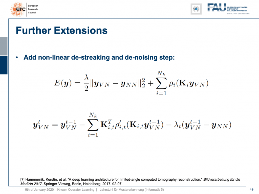
So, can we do more? Yes, there are even other things like so-called variational networks. This is work by Kobler, Pock, and Hammernik and they essentially showed that any kind of energy minimization can be mapped into a kind of unrolled, feed-forward problem. So, essentially an energy minimization can be solved by gradient descent. So, you essentially end up with an optimization problem that you seek to minimize. If you want to do that efficiently, you could essentially formulate this as a recurrent neural network. How did we deal with recurrent neural networks? Well, we unroll them. So any kind of energy minimization can be mapped into a feed-forward neural network, if you fix the number of iterations. This way, you can then take an energy minimization like this iterative reconstruction formula here or iterative denoising formula here and compute its gradient. If you do so, you will essentially end up with the previous image configuration minus the negative gradient direction. You do that and repeat this step by step.

那么，我們還能做更多嗎？ 是的，甚至還有其他一些東西，例如所謂的變分網絡。 這是Kobler，Pock和Hammernik的工作，他們實質上表明，任何一種能量最小化都可以映射為一種展開的前饋問題。 因此，基本上可以通過梯度下降來解決能量最小化問題。 因此，您最終會遇到要最小化的優化問題。 如果您想高效地做到這一點，則可以從本質上將其表述為遞歸神經網絡。 我們如何處理遞歸神經網絡？ 好吧，我們將它們展開。 因此，如果您固定迭代次數，則任何形式的能量最小化都可以映射到前饋神經網絡。 這樣，您就可以像此處的迭代重建公式或此處的迭代去噪公式那樣進行能量最小化，并計算其梯度。 如果這樣做，您將最終得到先前的圖像配置減去負梯度方向。 您這樣做，然后逐步重復此步驟。

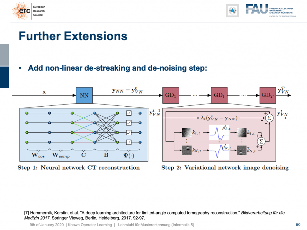
Here, we have a special solution because we combine it with our neural network reconstruction. We just want to learn an image enhancement step subsequently. So what we do is we take our neural network reconstruction and then hook up on the previous layers. There are T streaking or denoising steps that are trainable. They use compressed sensing theory. So, if you want to look into more details here, I recommend taking one of our image reconstruction classes. If you look into them you can see that there is this idea of compressing the image in a sparse domain. Here, we show that we can actually learn the transform that expresses the image contents in a sparse domain meaning that we can also get this new sparsifying transform and interpret it in a traditional signal processing sense.

在這里，我們有一個特殊的解決方案，因為我們將其與我們的神經網絡重建相結合。 我們只想隨后學習圖像增強步驟。 因此，我們要做的是我們進行神經網絡重建，然后連接到先前的層。 可以進行T條紋或去噪步驟。 他們使用壓縮感測理論。 因此，如果您想在此處了解更多詳細信息，建議您參加我們的圖像重建課程之一 。 如果查看它們，您會發現存在在稀疏域中壓縮圖像的想法。 在這里，我們表明，我們實際上可以學習在稀疏域中表示圖像內容的變換，這意味著我們也可以獲取此新的稀疏變換并以傳統的信號處理意義進行解釋。

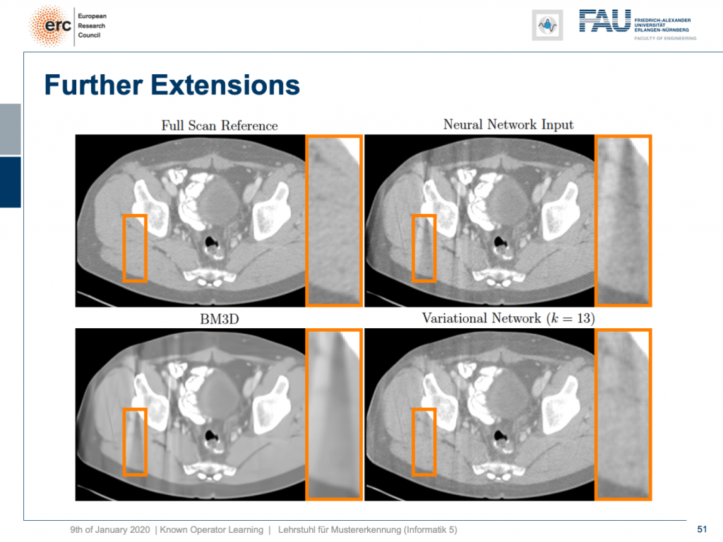
Let’s look at some results. Here, you can see that if we take the full scan reference, we get really an artifact-free image. Our neural network output with this reconstruction network that I showed earlier kind of is improved, but it still has these streak artifacts that you see on the top right. On the bottom left, you see the output of a denoising algorithm that is 3-D. So, this does denoising, but it still has problems with streaks. You can see that in our variational Network on the bottom right, the streaks are quite a bit suppressed. So, we really learn a transform based on the ideas of compressed sensing in order to remove those streaks. A very nice neural network that mathematically exactly models a compressed sensing reconstruction approach. So that’s exciting!

讓我們看一些結果。 在這里，您可以看到，如果我們使用完整的掃描參考，則實際上可以獲得無偽像的圖像。 我之前展示過的帶有該重構網絡的神經網絡輸出得到了改進，但是它仍然具有您在右上角看到的這些條紋痕跡。 在左下方，您會看到3-D去噪算法的輸出。 因此，這確實是去噪的，但是仍然存在條紋問題。 您可以看到在右下角的變化網絡中，條紋受到了很大的抑制。 因此，我們確實學習了基于壓縮感測思想的變換，以消除這些條紋。 一個非常不錯的神經網絡，可以在數學上精確地模擬壓縮感測重建方法。 真令人興奮！

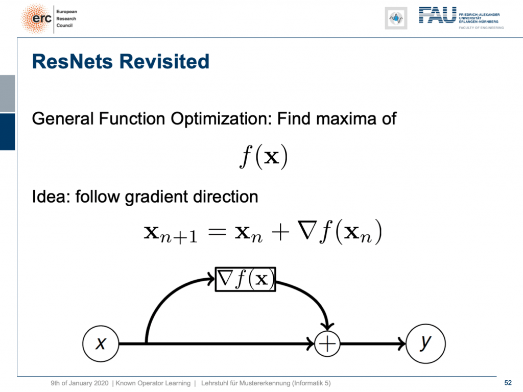
By the way, if you think of this energy minimization idea, then you also find the following interpretation: The energy minimization and this unrolling always lead to a ResNet because you take the previous configuration minus the negative gradient direction meaning that it’s the previous layers output plus the new layer’s configuration. So, this essentially means that ResNets can also be expressed in this kind of way. They always are the result of any kind of energy minimization problem. It could also be a maximization. In any case, we don’t even have to know whether it’s a maximization or minimization, but generally, if you have a function optimization, then you can always find the solution to this optimization process through a ResNet. So, you could argue that ResNets are also suited to find the optimization strategy for a completely unknown error function.

順便說一句，如果您想到這種能量最小化的想法，那么您還會發現以下解釋：能量最小化和這種展開始終會導致ResNet，因為您采用了先前的配置減去負梯度方向，這意味著它是先前的層輸出加上新層的配置。 因此，這實質上意味著ResNets也可以以這種方式表示。 它們始終是任何形式的能量最小化問題的結果。 這也可能是一個最大化。 無論如何，我們甚至都不必知道這是最大化還是最小化，但是通常，如果您進行了功能優化，則始終可以通過ResNet找到該優化過程的解決方案。 因此，您可能會說ResNets也適合為完全未知的誤差函數找到??優化策略。

Interesting, isn’t it? Well, there are a couple of more things that I want to tell you about these ideas of known operator learning. Also, we want to see more applications where we can apply this and maybe also some ideas on how the field of deep learning and machine learning will evolve over the next couple of months and years. So, thank you very much for listening and see you in the next and final video. Bye-bye!

有趣，不是嗎？ 好吧，關于這些關于已知操作員學習的想法，我想告訴您更多其他內容。 此外，我們希望看到更多可以在其中應用的應用程序，并且可能還需要一些關于深度學習和機器學習領域在未來幾個月和幾年中將如何發展的想法。 因此，非常感謝您的收聽，并在下一個也是最后一個視頻中見到您。 再見！

If you liked this post, you can find more essays here, more educational material on Machine Learning here, or have a look at our Deep LearningLecture. I would also appreciate a follow on YouTube, Twitter, Facebook, or LinkedIn in case you want to be informed about more essays, videos, and research in the future. This article is released under the Creative Commons 4.0 Attribution License and can be reprinted and modified if referenced. If you are interested in generating transcripts from video lectures try AutoBlog.

如果你喜歡這篇文章，你可以找到這里更多的文章 ，更多的教育材料，機器學習在這里 ，或看看我們的深入 學習 講座 。 如果您希望將來了解更多文章，視頻和研究信息，也歡迎關注YouTube ， Twitter ， Facebook或LinkedIn 。 本文是根據知識共享4.0署名許可發布的 ，如果引用，可以重新打印和修改。 如果您對從視頻講座中生成成績單感興趣，請嘗試使用AutoBlog 。

謝謝 (Thanks)

Many thanks to Weilin Fu, Florin Ghesu, Yixing Huang Christopher Syben, Marc Aubreville, and Tobias Würfl for their support in creating these slides.

非常感謝傅偉林，弗洛林·格蘇，黃宜興Christopher Syben，馬克·奧布雷維爾和托比亞斯·伍爾夫(TobiasWürfl)為創建這些幻燈片提供的支持。