📈Python金融系列 (📈Python for finance series)

Warning: There is no magical formula or Holy Grail here, though a new world might open the door for you.

警告 ： 這里沒有神奇的配方或圣杯，盡管新世界可能為您打開了大門。

📈Python金融系列 (📈Python for finance series)

1. Identifying Outliers

   識別異常值

2. Identifying Outliers — Part Two

   識別異常值-第二部分

3. Identifying Outliers — Part Three

   識別異常值-第三部分

4. Stylized Facts

   程式化的事實

5. Feature Engineering & Feature Selection

   特征工程與特征選擇

6. Data Transformation

   數據轉換

Following up the previous posts in these series, this time we are going to explore a real Technical Analysis (TA) in the financial market. For a very long time, I have been fascinated by the inner logic of TA called Volume Spread Analysis (VSA). I have found no articles on applying modern Machine learning on this time proving long-lasting technique. Here I am trying to throw out a minnow to catch a whale. If I could make some noise in this field, it was worth the time I spent on this article.

遵循這些系列中的先前文章，這次我們將探索金融市場中的實際技術分析(TA)。 很長時間以來，我一直著迷于TA的內部邏輯，即體積擴展分析(VSA)。 到目前為止，我還沒有發現有關應用現代機器學習的文章證明了其持久的技術。 在這里，我試圖扔一條小魚來捉鯨魚。 如果我能在這個領域引起一些轟動，那是值得我在本文上花費的時間。

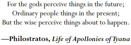
Especially, after I read David H. Weis’s Trades About to Happen, in his book he described:

特別是，在我閱讀David H. Weis的著作《 即將發生的交易》之后 ，他描述了：

“Instead of analyzing an array of indicators or algorithms, you should be able to listen to what any market says about itself.”1

“您不必分析各種指標或算法，而應該聽取任何市場對其自身的評價。”1

To closely listen to the market, as also well said from this quote below, just as it may not be possible to predict the future, it is also hard to neglect things about to happen. The key is to capture what is about to happen and follow the flow.

正如下面的引文所言，密切聽取市場意見，正如可能無法預測未來一樣，也很難忽略即將發生的事情。 關鍵是捕獲將要發生的事情并遵循流程。

But how to perceive things about to happen, a statement made long ago by Richard Wyckoff gives some clues:

但是，如何感知即將發生的事情， Richard Wyckoff很久以前發表的聲明給出了一些線索：

“Successful tape reading [chart reading] is a study of Force. It requires ability to judge which side has the greatest pulling power and one must have the courage to go with that side. There are critical points which occur in each swing just as in the life of a business or of an individual. At these junctures it seems as though a feather’s weight on either side would determine the immediate trend. Any one who can spot these points has much to win and little to lose.”2

“成功的磁帶閱讀[圖表閱讀]是對Force的研究。 它需要能夠判斷哪一方具有最大的拉動力，而一方必須有勇氣與那一方并駕齊驅。 就像企業或個人的生活一樣，每一個環節都有一些關鍵點。 在這些關頭，似乎兩側的羽毛重量將決定當前趨勢。 任何能夠發現這些點的人都將贏得很多，而損失卻很少。”2

But how to interpret the market behaviours? One of the eloquent description of market forces by Richard Wyckoff is very instructive:

但是，如何解釋市場行為呢？ 理查德·懷科夫 ( Richard Wyckoff )對市場力量的雄辯性描述之一很有啟發性：

“The market is like a slowly revolving wheel: Whether the wheel will continue to revolve in the same direction, stand still or reverse depends entirely upon the forces which come in contact with it hub and tread. even when the contact is broken, and nothing remains to affect its course, the wheel retains a certain impulse from the most recent dominating force, and revolves until it comes to a standstill or is subjected to other influences.”2

“市場就像一個緩慢旋轉的輪子：輪子將繼續沿相同方向旋轉，靜止還是反向旋轉，完全取決于與輪轂和胎面相接觸的力。 即使接觸斷開，也沒有影響其行程的方向盤，車輪仍會保留來自最新支配力的一定沖力，并旋轉直到其停止或受到其他影響。”2

David H. Weis gives a marvellous example of how to interpret the bars and relate them to the market behaviours. Through his construction of a hypothetical bar behaviour, every single bar becomes alive and rushes to tell you their stories.

戴維·H·韋斯(David H. Weis)提供了一個出色的例子，說明了如何解讀酒吧并將其與市場行為聯系起來。 通過構造一個假想的酒吧行為，每個酒吧都活著并爭先恐后地告訴您他們的故事。

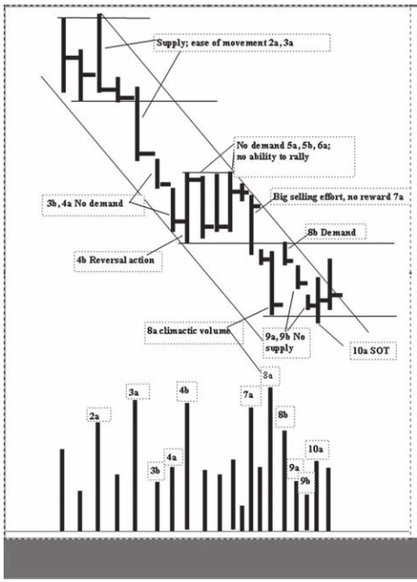
For all the details of the analysis, please refer to David’s book.

有關分析的所有詳細信息，請參閱David的書。

Before we dive deep into the code, it would be better to give a bit more background on Volume Spread Analysis (VSA). VSA is the study of the relationship between volume and price to predict market direction by following the professional traders, so-called market maker. All the interpretations of market behaviours follow 3 basic laws:

在深入研究代碼之前，最好對體積擴展分析(VSA)有所了解。 VSA是對數量和價格之間關系的研究，旨在通過跟隨專業交易者(所謂的做市商)來預測市場方向。 市場行為的所有解釋都遵循3個基本定律：

• The Law of Supply and Demand
  供求法則
• The Law of Effort vs. Results
  努力法則與結果
• The Law of Cause and Effect
  因果定律

There are also three big names in VSA’s development history.

VSA的發展歷史上也有三大名聲。

• Jesse Livermore
  杰西·利佛摩
• Richard Wyckoff
  理查德·威科夫(Richard Wyckoff)
• Tom Williams
  湯姆·威廉姆斯

And tons of learning materials can be found online. For a beginner, I would recommend the following 2 books.

大量的學習資料可以在網上找到。 對于初學者，我建議以下2本書。

1. Master the Markets by Tom Williams

   湯姆·威廉姆斯(Tom Williams) 掌握市場

2. Trades About to Happen by David H. Weis

   David H. Weis 即將發生的交易

Also, if you only want to have a quick peek on this topic, there is a nice article on VSA from here.

另外，如果您只想快速瀏覽一下此主題，可以在此處找到有關VSA的不錯的文章。

One of the great advantages of Machine learning / Deep learning lies on the no need for feature engineering. The basic of VSA is, as said in its name, volume, the spread of price range, location of the close related to the change of stock price in a bar.

機器學習/深度學習的一大優勢在于無需特征工程。 正如其名稱中所述，VSA的基本原理是數量，價格范圍的價差，與條形圖的股價變化相關的收盤位置。

These features can be defined as:

這些功能可以定義為：

• Volume: pretty straight forward
  數量：挺直的
• Range/Spread: Difference between high and close
  范圍/價差：最高價和收市價之間的差異
• Closing Price Relative to Range: Is the closing price near the top or the bottom of the price bar?
  收盤價相對于范圍：收盤價是否在價格柱的頂部或底部附近？
• The change of stock price: pretty straight forward
  股票價格的變化：很簡單

There are many terminologies created by Richard Wyckoff, like Sign of strength (SOS), Sign of weakness (SOW) etc.. However, most of those terminologies are purely the combination of those 4 basic features. I don’t believe that, with deep learning, over-engineering features is a sensible thing to do. Considering one of the advantages of deep learning is that it completely automates what used to be the most crucial step in a machine-learning workflow: feature engineering. The thing we need to do is to tell the algorithm where to look at, rather than babysitting them step by step. Without further ado, let’s dive into the code.

理查德·懷科夫(Richard Wyckoff)創建了許多術語 ，例如“強勢跡象(SOS)”，“弱勢跡象(SOW)”等。但是，這些術語中的大多數純粹是這四個基本特征的組合。 我不認為通過深度學習，過度設計功能不是明智的選擇。 考慮到深度學習的優點之一是它可以完全自動化機器學習工作流程中最關鍵的步驟：特征工程。 我們需要做的是告訴算法要看的地方，而不是一步一步地照顧他們。 事不宜遲，讓我們深入研究代碼。

1.數據準備 (1. Data preparation)

For consistency, in all the 📈Python for finance series, I will try to reuse the same data as much as I can. More details about data preparation can be found here, here and here.

為了保持一致性，在所有Python金融系列叢書中 ，我將盡量重用相同的數據。 有關數據準備的更多詳細信息，可以在此處 ， 此處和此處找到 。

#import all the libraries
import pandas as pd
import numpy as np
import seaborn as sns 
import yfinance as yf  #the stock data from Yahoo Financeimport matplotlib.pyplot as plt #set the parameters for plotting
plt.style.use('seaborn')
plt.rcParams['figure.dpi'] = 300#define a function to get data
def get_data(symbols, begin_date=None,end_date=None):
    df = yf.download('AAPL', start = '2000-01-01',
                     auto_adjust=True,#only download adjusted data
                     end= '2010-12-31') 
    #my convention: always lowercase
    df.columns = ['open','high','low',
                  'close','volume'] 
    
    return df
prices = get_data('AAPL', '2000-01-01', '2010-12-31')   
prices.head()

?提示！ (?Tip!)

The data we download this time is adjusted data from yfinance by setting the auto_adjust=True. If you have access to tick data, by all means. It would be much better with tick data as articulated from Advances in Financial Machine Learning by Marcos Prado. Anyway, 10 years adjusted data only gives 2766 entries, which is far from “Big Data”.

我們這次下載的數據是 通過設置 auto_adjust=True 從 yfinance 調整的數據 。 如果可以訪問滴答數據，請務必。 剔除的報價數據會更好 Marcos Prado 在金融機器學習中 的 進展 。 無論如何，經過10年調整的數據僅提供2766條記錄，與“大數據”相去甚遠。

2.特征工程 (2. Feature Engineering)

The key point of combining VSA with modern data science is through reading and interpreting the bars' own actions, one (hopefully algorithm) can construct a story of the market behaviours. The story might not be easily understood by a human, but works in a sophisticated way.

將VSA與現代數據科學相結合的關鍵點在于，通過閱讀和解釋條形自身的行為，一個(希望是一種算法)可以構建一個關于市場行為的故事。 這個故事可能不容易為人類所理解，而是以一種復雜的方式進行。

Volume in conjunction with the price range and the position of the close is easy to be expressed by code.

交易量，價格范圍和收盤位置很容易用代碼表示。

• Volume: pretty straight forward
  數量：挺直的
• Range/Spread: Difference between high and close
  范圍/價差：最高價和收市價之間的差異

def price_spread(df):
    return (df.high - df.low)

• Closing Price Relative to Range: Is the closing price near the top or the bottom of the price bar?
  收盤價相對于范圍：收盤價是否在價格柱的頂部或底部附近？

def close_location(df):
    return (df.high - df.close) / (df.high - df.low)#o indicates the close is the high of the day, and 1 means close
#is the low of the day and the smaller the value, the closer the #close price to the high.

• The change of stock price: pretty straight forward
  股票價格的變化：很簡單

Now comes the tricky part,

現在是棘手的部分，

“When viewed in a larger context, some of the price bars take on a new meaning.”

“從更大的角度來看，某些價格柱具有新的含義。”

That means to see the full pictures, we need to observe those 4 basic features under a different time scale.

這意味著要查看完整圖片，我們需要在不同的時間范圍內觀察這4個基本功能。

To do that, we need to reconstruct a High(H), Low(L), Close(C) and Volume(V) bar at varied time span.

為此，我們需要在不同的時間跨度上重建高(H)，低(L)，關閉(C)和體積(V)條。

def create_HLCV(i): 
'''
#i: days
#as we don't care about open that much, that leaves volume, 
#high,low and close
'''     df = pd.DataFrame(index=prices.index)    df[f'high_{i}D'] = prices.high.rolling(i).max()
    df[f'low_{i}D'] = prices.low.rolling(i).min()
    df[f'close_{i}D'] = prices.close.rolling(i).\
                        apply(lambda x:x[-1]) 
    # close_2D = close as rolling backwards means today is 
    #literally, the last day of the rolling window.
    df[f'volume_{i}D'] = prices.volume.rolling(i).sum()
    
    return df

next step, create those 4 basic features based on a different time scale.

下一步，根據不同的時間范圍創建這4個基本功能。

def create_features(i):
    df = create_HLCV(i)
    high = df[f'high_{i}D']
    low = df[f'low_{i}D']
    close = df[f'close_{i}D']
    volume = df[f'volume_{i}D']
    
    features = pd.DataFrame(index=prices.index)
    features[f'volume_{i}D'] = volume
    features[f'price_spread_{i}D'] = high - low
    features[f'close_loc_{i}D'] = (high - close) / (high - low)
    features[f'close_change_{i}D'] = close.diff()
    
    return features

The time spans that I would like to explore are 1, 2, 3 days and 1 week, 1 month, 2 months, 3 months, which roughly are [1,2,3,5,20,40,60] days. Now, we can create a whole bunch of features,

我想探索的時間范圍是1、2、3天和1周，1個月，2個月，3個月，大約是[1,2,3,5,20,40,60]天。 現在，我們可以創建很多功能，

def create_bunch_of_features():
    days = [1,2,3,5,20,40,60]
    bunch_of_features = pd.DataFrame(index=prices.index)
    for day in days:
        f = create_features(day)
        bunch_of_features = bunch_of_features.join(f)
    
    return bunch_of_featuresbunch_of_features = create_bunch_of_features()
bunch_of_features.info()

To make things easy to understand, our target outcome will only be the next day’s return.

為了使事情易于理解，我們的目標結果將僅是第二天的退貨。

# next day's returns as outcomes
outcomes = pd.DataFrame(index=prices.index)
outcomes['close_1'] = prices.close.pct_change(-1)

3.特征選擇 (3. Feature Selection)

Let’s have a look at how those features correlated with outcomes, the next day’s return.

讓我們看一下這些功能與結果，第二天的收益如何相關。

corr = bunch_of_features.corrwith(outcomes.close_1)
corr.sort_values(ascending=False).plot.barh(title = 'Strength of Correlation');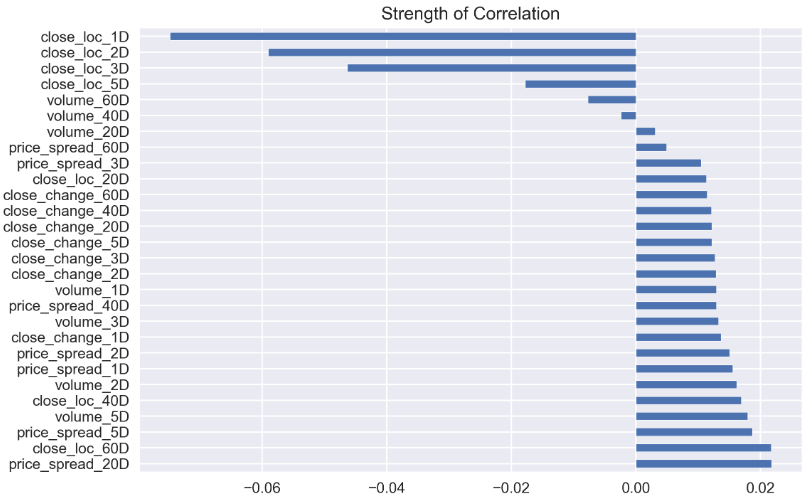

It is hard to say there are some correlations, as all the numbers are well below 0.8.

很難說存在一些相關性，因為所有數字都遠低于0.8。

corr.sort_values(ascending=False)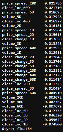

Next, let’s see how those features related to each other.

接下來，讓我們看看這些功能如何相互關聯。

corr_matrix = bunch_of_features.corr()

Instead of making heatmap, I am trying to use Seaborn’s Clustermap to cluster row-wise or col-wise to see if there is any pattern emerges. Seaborn’s Clustermap function is great for making simple heatmaps and hierarchically-clustered heatmaps with dendrograms on both rows and/or columns. This reorganizes the data for the rows and columns and displays similar content next to one another for even more depth of understanding the data. A nice tutorial about cluster map can be found here. To get a cluster map, all you need is actually one line of code.

我沒有制作熱圖，而是嘗試使用Seaborn的Clustermap對行或逐行進行聚類，以查看是否出現任何模式。 Seaborn的Clustermap功能非常適用于制作簡單的熱圖和在行和/或列上均具有樹狀圖的層次集群的熱圖。 這將重新組織行和列的數據，并相鄰顯示相似的內容，以進一步了解數據。 可以在這里找到有關集群映射的很好的教程。 要獲得集群圖，實際上只需要一行代碼。

sns.clustermap(corr_matrix)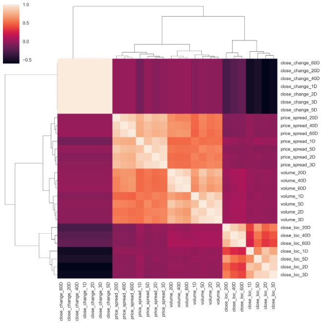

If you carefully scrutinize the graph, some conclusions can be drawn:

如果仔細檢查圖形，可以得出一些結論：

1. Price spread closely related to the volume, as clearly shown at the centre of the graph.
   價格點差與交易量密切相關，如圖表中心所示。
2. And the location of close related to each other at different timespan, as indicated at the bottom right corner.
   并且關閉位置在不同的時間范圍內彼此相關，如右下角所示。
3. From the pale colour of the top left corner, close price change does pair with itself, which makes perfect sense. However, it is a bit random as no cluster pattern at varied time scale. I would expect that 2Days change should be paired with 3Days change.
   從左上角的淺色開始，接近的價格變化與自身匹配，這是很合理的。 但是，由于在變化的時間尺度上沒有群集模式，因此它有點隨機。 我希望2天的更改應與3天的更改配對。

The randomness of the close price difference could thank to the characteristics of the stock price itself. Simple percentage return might be a better option. This can be realized by modifying the close diff() to close pct_change().

收盤價差的隨機性可以歸功于股票價格本身的特征。 簡單的百分比回報可能是更好的選擇。 這可以通過將close diff()修改為close pct_change() 。

def create_features_v1(i):
    df = create_HLCV(i)
    high = df[f'high_{i}D']
    low = df[f'low_{i}D']
    close = df[f'close_{i}D']
    volume = df[f'volume_{i}D']
    
    features = pd.DataFrame(index=prices.index)
    features[f'volume_{i}D'] = volume
    features[f'price_spread_{i}D'] = high - low
    features[f'close_loc_{i}D'] = (high - close) / (high - low)
    #only change here
    features[f'close_change_{i}D'] = close.pct_change()
    
    return features

and do everything again.

然后再做一遍。

def create_bunch_of_features_v1():
    days = [1,2,3,5,20,40,60]
    bunch_of_features = pd.DataFrame(index=prices.index)
    for day in days:
        f = create_features_v1(day)#here is the only difference
        bunch_of_features = bunch_of_features.join(f)
    
    return bunch_of_featuresbunch_of_features_v1 = create_bunch_of_features_v1()#check the correlation
corr_v1 = bunch_of_features_v1.corrwith(outcomes.close_1)
corr_v1.sort_values(ascending=False).plot.barh( title = 'Strength of Correlation')

a little bit different, but not much!

有點不同，但是沒有太大關系！

corr_v1.sort_values(ascending=False)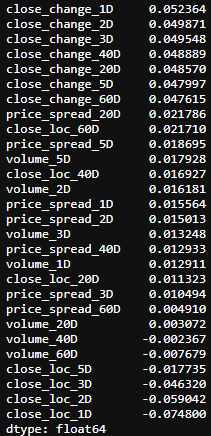

What happens to the correlation between features?

特征之間的相關性會發生什么？

corr_matrix_v1 = bunch_of_features_v1.corr()
sns.clustermap(corr_matrix_v1, cmap='coolwarm', linewidth=1)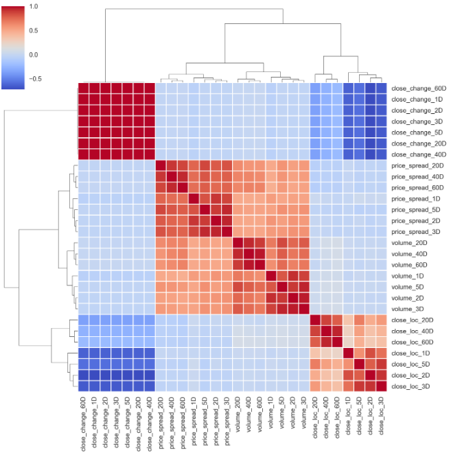

Well, the pattern remains unchanged. Let’s change the default method from “average” to “ward”. These two methods are similar, but “ward” is more like K-MEANs clustering. A nice tutorial on this topic can be found here.

好吧，模式保持不變。 讓我們將默認方法從“平均值”更改為“病房”。 這兩種方法相似，但是“ ward”更像是K-MEAN聚類。 可以在這里找到有關該主題的不錯的教程。

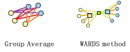
sns.clustermap(corr_matrix_v1, cmap='coolwarm', linewidth=1,
                         method='ward')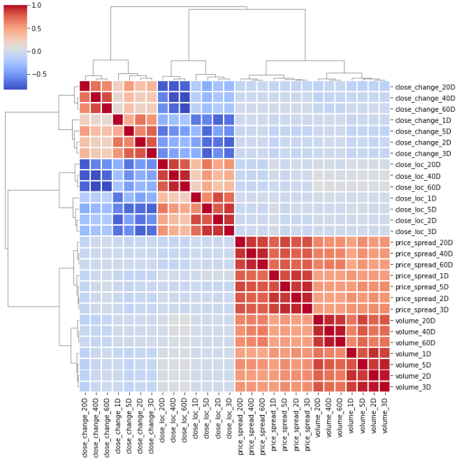

To select features, we want to pick those that have the strongest, most persistent relationships to the target outcome. At the meantime, to minimize the amount of overlap or collinearity in your selected features to avoid noise and waste of computer power. For those features that paired together in a cluster, I only pick the one that has a stronger correlation with the outcome. By just looking at the cluster map, a few features are picked out.

要選擇特征，我們要選擇與目標結果之間關系最牢固，最持久的特征。 同時，為了最大程度地減少所選功能中的重疊或共線性，避免產生噪音和計算機電源浪費。 對于在集群中配對在一起的那些特征，我只選擇與結果相關性更強的那些特征。 通過僅查看聚類圖，就可以挑選出一些功能。

deselected_features_v1 = ['close_loc_3D','close_loc_60D',
                       'volume_3D', 'volume_60D',
                       'price_spread_3D','price_spread_60D',
                       'close_change_3D','close_change_60D']selected_features_v1 = bunch_of_features.drop \
(labels=deselected_features_v1, axis=1)

Next, we are going to take a look at pair-plot, A pair plot is a great method to identify trends for follow-up analysis, allowing us to see both distributions of single variables and relationships between multiple variables. Again, all we need is a single line of code.

接下來，我們將看一下配對圖， 配對圖是識別趨勢以進行后續分析的好方法，它使我們既可以看到單個變量的分布又可以看到多個變量之間的關系。 同樣，我們只需要一行代碼。

sns.pairplot(selected_features_v1)

The graph is overwhelming and hard to see. Let’s take a small group as an example.

該圖是壓倒性的，很難看到。 讓我們以一個小組為例。

selected_features_1D_list = ['volume_1D', 'price_spread_1D',\         'close_loc_1D', 'close_change_1D']selected_features_1D = selected_features_v1\
                       [selected_features_1D_list]sns.pairplot(selected_features_1D)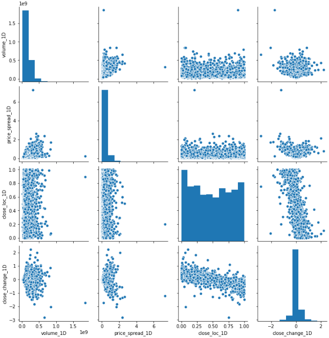

There are two things I noticed immediately, one is there are outliers and another is the distribution are no way close to normal.

我立即注意到兩件事，一是存在離群值，二是分布與正常值相差無幾。

Let’s deal with the outliers for now. In order to do everything in one go, I will join the outcome with features and remove outliers together.

現在讓我們處理異常值。 為了一次性完成所有工作，我將結果與功能結合在一起，并將異常值一起移除。

features_outcomes = selected_features_v1.join(outcomes)
features_outcomes.info()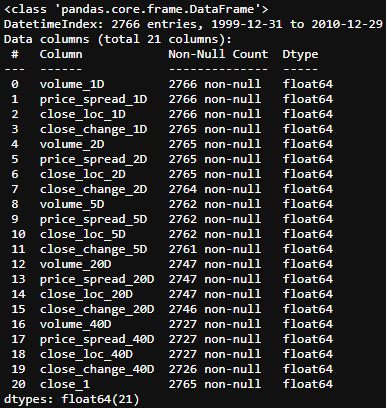

I will use the same method described here, here and here to remove the outliers.

我將使用此處 ， 此處和此處所述的相同方法來刪除異常值。

stats = features_outcomes.describe()
def get_outliers(df, i=4): 
    #i is number of sigma, which define the boundary along mean
    outliers = pd.DataFrame()
    
    for col in df.columns:
        mu = stats.loc['mean', col]
        sigma = stats.loc['std', col]
        condition = (df[col] > mu + sigma * i) | (df[col] < mu - sigma * i) 
        outliers[f'{col}_outliers'] = df[col][condition]
    
    return outliersoutliers = get_outliers(features_outcomes, i=1)
outliers.info()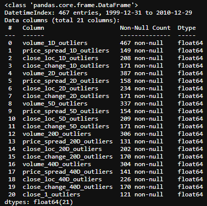

I set 1 standard deviation as the boundary to dig out most of the outliers. Then remove all the outliers along with the NaN values.

我將1個標準差設置為邊界，以挖掘出大多數異常值。 然后刪除所有異常值以及NaN值。

features_outcomes_rmv_outliers = features_outcomes.drop(index = outliers.index).dropna()
features_outcomes_rmv_outliers.info()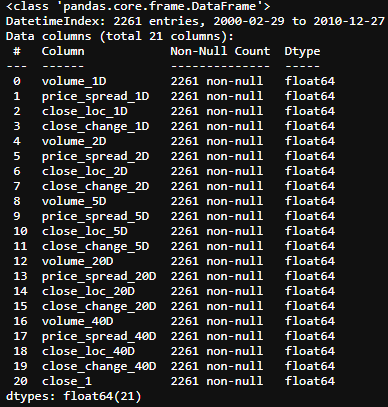

With the outliers removed, we can do the pair plot again.

除去異常值后，我們可以再次繪制對圖。

sns.pairplot(features_outcomes_rmv_outliers, vars=selected_features_1D_list);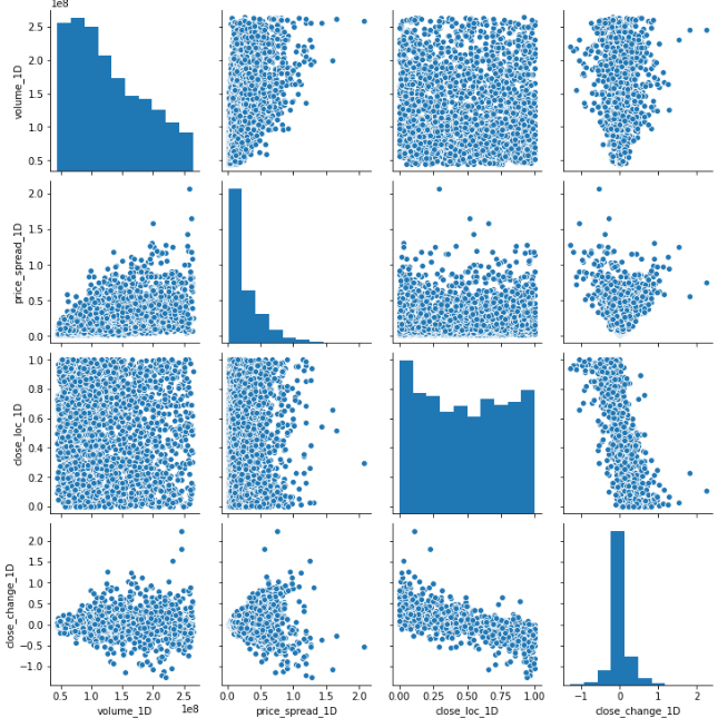

Now, the plots are looking much better, but it is barely to draw any useful conclusions. It would be nice to see which spots are down moves and which are up moves in conjunction with those features. I can extract the sign of stock price change and add an extra dimension to the plots.

現在，這些圖看起來好多了，但是幾乎沒有得出任何有用的結論。 很高興看到哪些點向下移動，哪些點向上移動以及這些功能。 我可以提取股票價格變化的跡象，并為圖添加額外的維度。

features_outcomes_rmv_outliers['sign_of_close'] = features_outcomes_rmv_outliers['close_1'].apply(np.sign)

Now, let’s re-plot the pairplot() again with a bit of tweak to make the graph pretty.

現在，讓我們通過一些調整再次重新繪制pairplot() ，以使圖表更漂亮。

sns.pairplot(features_outcomes_rmv_outliers, 
             vars=selected_features_1D_list,
             diag_kind='kde',
             palette='husl', hue='sign_of_close',
             markers = ['*', '<', '+'], 
             plot_kws={'alpha':0.3});#transparence:0.3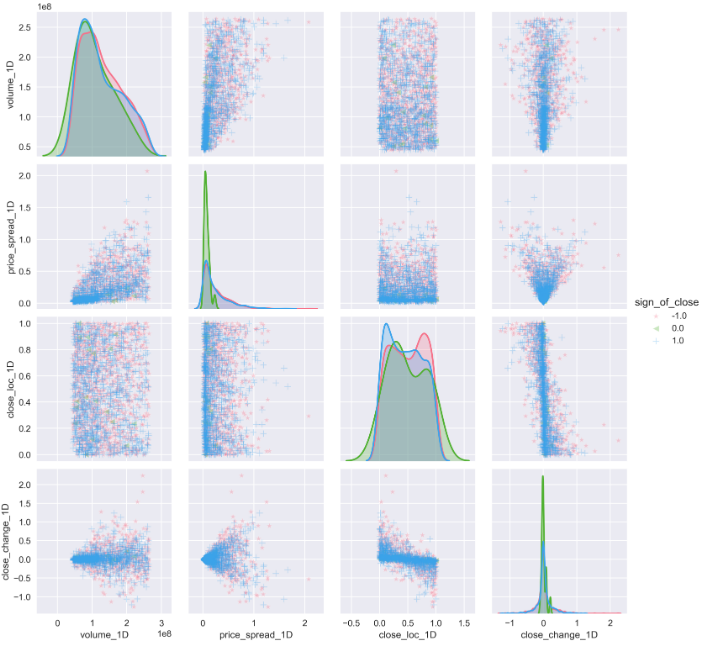

Now, it looks much better. Clearly, when the prices go up, they (the blue spot) are denser and aggregate at a certain location. Whereas on down days, they spread everywhere.

現在，它看起來好多了。 顯然，當價格上漲時，它們(藍色點)在某個位置更密集且聚集在一起。 而在低迷時期，它們無處不在。

I would really appreciate it if you could shed some light on the pair plot and leave your comments below, thanks.

如果您能對結對圖有所了解并在下面留下您的評論，我將非常感激。

Here is the summary of all the codes used in this article:

這是本文中使用的所有代碼的摘要：

#import all the libraries
import pandas as pd
import numpy as np
import seaborn as sns 
import yfinance as yf  #the stock data from Yahoo Financeimport matplotlib.pyplot as plt #set the parameters for plotting
plt.style.use('seaborn')
plt.rcParams['figure.dpi'] = 300#define a function to get data
def get_data(symbols, begin_date=None,end_date=None):
    df = yf.download('AAPL', start = '2000-01-01',
                     auto_adjust=True,#only download adjusted data
                     end= '2010-12-31') 
    #my convention: always lowercase
    df.columns = ['open','high','low',
                  'close','volume'] 
    
    return dfprices = get_data('AAPL', '2000-01-01', '2010-12-31')#create some features
def create_HLCV(i):#as we don't care open that much, that leaves volume, 
#high,low and closedf = pd.DataFrame(index=prices.index)
    df[f'high_{i}D'] = prices.high.rolling(i).max()
    df[f'low_{i}D'] = prices.low.rolling(i).min()
    df[f'close_{i}D'] = prices.close.rolling(i).\
                        apply(lambda x:x[-1]) 
    # close_2D = close as rolling backwards means today is 
    # literly the last day of the rolling window.
    df[f'volume_{i}D'] = prices.volume.rolling(i).sum()
    
    return dfdef create_features_v1(i):
    df = create_HLCV(i)
    high = df[f'high_{i}D']
    low = df[f'low_{i}D']
    close = df[f'close_{i}D']
    volume = df[f'volume_{i}D']
    
    features = pd.DataFrame(index=prices.index)
    features[f'volume_{i}D'] = volume
    features[f'price_spread_{i}D'] = high - low
    features[f'close_loc_{i}D'] = (high - close) / (high - low)
    features[f'close_change_{i}D'] = close.pct_change()
    
    return featuresdef create_bunch_of_features_v1():
'''
the timespan that i would like to explore 
are 1, 2, 3 days and 1 week, 1 month, 2 month, 3 month
which roughly are [1,2,3,5,20,40,60]
'''
    days = [1,2,3,5,20,40,60]
    bunch_of_features = pd.DataFrame(index=prices.index)
    for day in days:
        f = create_features_v1(day)
        bunch_of_features = bunch_of_features.join(f)
    
    return bunch_of_featuresbunch_of_features_v1 = create_bunch_of_features_v1()#define the outcome target
#here， to make thing easy to understand, i will only try to predict #the next days's return
outcomes = pd.DataFrame(index=prices.index)# next day's returns
outcomes['close_1'] = prices.close.pct_change(-1)#decide which features are abundant from cluster map
deselected_features_v1 = ['close_loc_3D','close_loc_60D',
                       'volume_3D', 'volume_60D',
                       'price_spread_3D','price_spread_60D',
                       'close_change_3D','close_change_60D']
selected_features_v1 = bunch_of_features_v1.drop(labels=deselected_features_v1, axis=1)#join the features and outcome together to remove the outliers
features_outcomes = selected_features_v1.join(outcomes)
stats = features_outcomes.describe()#define the method to identify outliers
def get_outliers(df, i=4): 
    #i is number of sigma, which define the boundary along mean
    outliers = pd.DataFrame()
    
    for col in df.columns:
        mu = stats.loc['mean', col]
        sigma = stats.loc['std', col]
        condition = (df[col] > mu + sigma * i) | (df[col] < mu -   sigma * i) 
        outliers[f'{col}_outliers'] = df[col][condition]
    
    return outliersoutliers = get_outliers(features_outcomes, i=1)#remove all the outliers and Nan value
features_outcomes_rmv_outliers = features_outcomes.drop(index = outliers.index).dropna()

I know this article goes too long, I am better off leaving it here. In the next article, I will do a data transformation to see if I have a way to fix the issue of distribution. Stay tuned!

我知道這篇文章太長了，最好把它留在這里。 在下一篇文章中，我將進行數據轉換，以查看是否有辦法解決分發問題。 敬請關注！