The code for this project can be found at my GitHub.

該項目的代碼可以在我的GitHub上找到 。

介紹 (Introduction)

The goal of this project was to analyse historic stock/inventory data to decide how much stock of each item a retailer should hold in the future. When deciding which historic data to use I came across a great blog post by Nhan Tran on Towards Data Science. This post provided me with the data set I was looking for. The best thing about this post was that it gave a brief outline of a project, but no code. This meant I had to write all the code myself from scratch (which is good practice), yet I could check my answers at each stage using the landmarks in Nhan Tran’s blog post.

該項目的目的是分析歷史庫存/庫存數據，以確定零售商將來應持有的每件商品多少庫存。 在決定使用哪些歷史數據時，我遇到了Nhan Tran撰寫的一篇很棒的博客文章 ，名為Towards Data Science 。 這篇文章為我提供了我想要的數據集 。 關于這篇文章的最好的事情是它給出了一個項目的簡要概述，但是沒有代碼。 這意味著我必須自己重新編寫所有代碼(這是一種很好的做法)，但是我可以使用Nhan Tran 博客文章中的地標在每個階段檢查答案。

I completed the project using Python in a Jupyter Notebook.

我在Jupyter Notebook中使用Python完成了該項目 。

技術目標 (Technical Goal)

To give (with 95% confidence) a lower and upper bound for how many pairs of Men’s shoes, of each size, a shop in the United States should stock for any given month.

為了給(具有95％的置信度)上下限，確定每個給定月份在美國的商店應存多少種每種尺寸的男鞋。

設置筆記本并導入數據 (Setting Up the Notebook and Importing the Data)

First I read through the project and decided which libraries I would need to use. I then imported those libraries into my notebook:

首先，我通讀該項目，并確定需要使用哪些庫。 然后，我將這些庫導入到筆記本中：

Note: some of these libraries I didn’t foresee using and I went back and added them as and when I needed them.

注意 ：其中一些我沒有預見到的庫，我回去并在需要時添加它們。

Next I downloaded the data set and imported it into my notebook using read_csv() from the pandas library:

接下來，我從pandas庫中使用read_csv()下載了數據集并將其導入到筆記本中：

sales = pd.read_csv("Al-Bundy_raw-data.csv")

檢查和清理數據 (Inspecting and Cleaning the Data)

Before beginning the project I inspected the DataFrame.

在開始項目之前，我檢查了DataFrame。

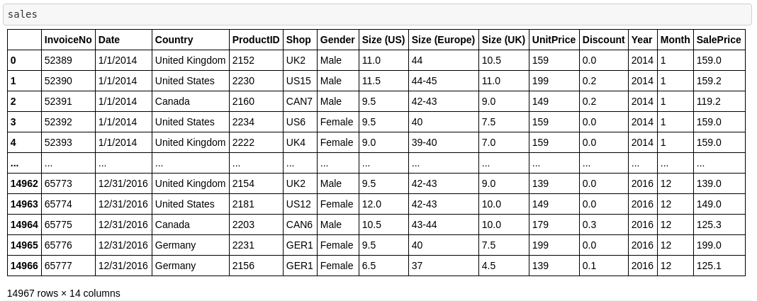
Each row on the data set represent a pair of shoes that had been sold.

數據集的每一行代表一雙已售出的鞋子。

I then inspected the data types of each column to ensure they made sense.

然后，我檢查了每一列的數據類型，以確保它們有意義。

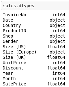
I then changed the 'Date' datatype from object to datetime using the following code:

然后我改變了'Date'數據類型從object到datetime使用以下代碼：

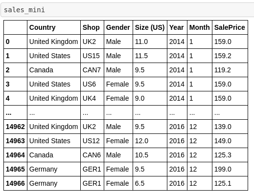
sales['Date'] = pd.to_datetime(sales['Date'])

Based on the specific goal of this project I then decided to drop any columns that would not be relevant during this analysis. I dropped the European and UK size equivalents as only one size type was needed, and since I was focusing on US stores in particular I decided to keep US sizes to analyse. I dropped the Date column as I already had the month and year data in separate columns and did not need to be more specific than this. I also dropped the Product ID, Invoice Number, Discount and Sale Price as they were either irrelevant or their effect on stock levels was beyond the scope of this project. I achieved this using the following code:

基于此項目的特定目標，我然后決定刪除此分析期間不相關的任何列。 因為只需要一種尺碼類型，所以我放棄了歐洲和英國的尺碼對應關系，并且由于我特別關注美國商店，因此我決定保留美國尺碼進行分析。 我刪除了Date列，因為我已經在不同的列中包含了月份和年份數據，并且不需要比此更具體。 我還刪除了產品ID，發票編號，折扣和銷售價格，因為它們無關緊要或它們對庫存水平的影響超出了此項目的范圍。 我使用以下代碼實現了這一點：

sales_mini = sales.drop(['InvoiceNo', 'ProductID','Size (Europe)', 'Size (UK)', 'UnitPrice', 'Discount', 'Date'], axis=1)

This left me with a more streamlined and easier to read DataFrame to analyse.

這為我提供了更簡化和更易于讀取的DataFrame進行分析。

數據分析與可視化 (Data Analysis and Visualisation)

I now decided to concentrate on an even smaller set of data, although this may have sacrificed accuracy by using a smaller data set, it also may have gained accuracy by using the most relevant data available.

我現在決定集中精力于更小的數據集，盡管使用較小的數據集可能會犧牲準確性，但使用可用的最相關數據也可能會提高準確性。

To do this I first created a new DataFrame of only Male shoes, using the following code:

為此，我首先使用以下代碼創建了一個僅男鞋的新數據框：

sales_mini_male = sales_mini[sales_mini['Gender'] == 'Male']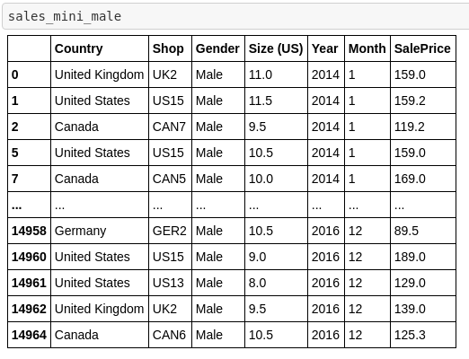

I then selected all of the rows where the shoes were sold in the United States in 2016, in order to make the data as relevant to our goal as possible. I achieved this with the following code:

然后，我選擇了2016年在美國銷售鞋子的所有行，以使數據盡可能與我們的目標相關。 我通過以下代碼實現了這一點：

male_2016 = sales_mini_male[sales_mini_male['Year']==2016]
male_us_2016 = male_2016[male_2016['Country']=='United States']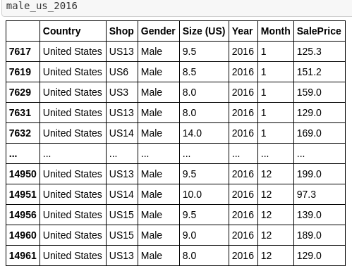

The above DataFrame doesn’t make it clear which shoe sizes were the most frequent. To find out which shoe sizes were, I created a pivot table, analysing how many shoes of each size were sold each month (since people may be more likely to buy shoes in some months that others). I achieved this using the following code:

上面的DataFrame并不清楚哪個鞋號是最常見的。 為了找出哪種尺寸的鞋，我創建了一個數據透視表，分析了每個月售出每種尺寸的鞋的數量(因為人們可能會在幾個月內購買其他鞋的可能性更高)。 我使用以下代碼實現了這一點：

male_us_2016_by_month = pd.pivot_table(male_us_2016, values='Country', index=['Size (US)'], columns=['Month'], fill_value=0, aggfunc=len)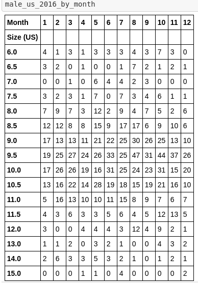

Albeit more useful, the above table is still difficult to read. To solve this problem I imported the seaborn library, and displayed the pivot table as a heat map.

上表雖然更有用，但仍然很難閱讀。 為了解決此問題，我導入了seaborn庫，并將數據透視表顯示為熱圖。

plt.figure(figsize=(16, 6))
male_us_2016_by_month_heatmap = sns.heatmap(male_us_2016_by_month, annot=True, fmt='g', cmap='Blues')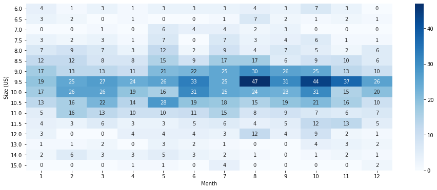

This heat map indicates that demand for shoes, across different sizes is likely to be a normal distribution. This makes sense when thinking logically, as few people have extremely small or extremely large feet, but many have a shoe size somewhere in between. I then illustrated this even clearer by plotting the total yearly demand for each size in a bar chart.

該熱圖表明，不同尺寸的鞋子需求可能是正態分布。 從邏輯上考慮時，這是有道理的，因為很少有人腳很小或太大，但是很多人的鞋子介于兩者之間。 然后，我通過在條形圖中繪制每種尺寸的年度總需求來說明這一點。

male_us_2016_by_month_with_total = pd.pivot_table(male_us_2016, values='Country', index=['Size (US)'], columns=['Month'], fill_value=0, margins=True, margins_name='Total', aggfunc=len)
male_us_2016_by_month_with_total_right = male_us_2016_by_month_with_total.iloc[:-1, :]
male_us_2016_by_month_with_total_right = male_us_2016_by_month_with_total_right.reset_index()
male_us_2016_total_by_size = male_us_2016_by_month_with_total_right[['Size (US)', 'Total']]
male_us_2016_by_size_plot = male_us_2016_total_by_size.plot.bar(x='Size (US)',y='Total', legend=False)
male_us_2016_by_size_plot.set_ylabel("Frequency")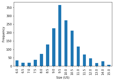

Although this analysis would be useful to a retailer, this is just an overview of what happened in 2016.

盡管此分析對零售商有用，但這只是2016年情況的概述。

學生考試 (Student’s T-test)

To give a prediction on future levels of demand, with a given degree of confidence, I performed a statistical test on the data. Since the remaining relevant data was a small data set, and that it closely represented a normal distribution, I decided a Student’s T-test would be the most relevant.

為了以給定的可信度預測未來的需求水平，我對數據進行了統計檢驗。 由于剩余的相關數據是一個很小的數據集，并且它緊密地代表了正態分布，因此我認為學生的T檢驗將是最相關的。

First I found the t-value to be used in a 2-tailed test finding 95% confidence intervals (note: 0.5 had to be divided by 2 to get 0.025 as the test is 2-tailed).

首先，我發現t值用于2尾檢驗中，發現置信區間為95％(注意：由于2尾檢驗，必須將0.5除以2才能得到0.025)。

t_value = stats.t.ppf(1-0.025,11)

I then used this t-value to calculate the ‘Margin Error’ and displayed this along with other useful aggregates in the following table using the following code:

然后，我使用此t值來計算“邊距誤差”，并使用以下代碼在下表中將其與其他有用的匯總一起顯示：

male_us_2016_agg = pd.DataFrame()
male_us_2016_agg['Size (US)'] = male_us_2016_by_month_with_total['Size (US)']
male_us_2016_agg['Mean'] = male_us_2016_by_month_with_total.mean(1)
male_us_2016_agg['Standard Error'] = male_us_2016_by_month_with_total.sem(1)
male_us_2016_agg['Margin Error'] = male_us_2016_agg['Standard Error'] * t_value
male_us_2016_agg['95% CI Lower Bound'] = male_us_2016_agg['Mean'] - male_us_2016_agg['Margin Error']
male_us_2016_agg['95% CI Upper Bound'] = male_us_2016_agg['Mean'] + male_us_2016_agg['Margin Error']

零售商友好輸出 (Retailer Friendly Output)

I then decided to re-present my data in a more easy to understand format. I made sure python did as much of the work for me here as possible to ensure my code was efficient and easy to replicate and scale.

然后，我決定以一種更易于理解的格式重新呈現我的數據。 我確保python在這里為我做了盡可能多的工作，以確保我的代碼高效且易于復制和擴展。

conclusion = pd.DataFrame()
conclusion['Size (US)'] = male_us_2016_agg['Size (US)']
conclusion['Lower Bound'] = male_us_2016_agg['95% CI Lower Bound'].apply(np.ceil)
conclusion['Lower Bound'] = conclusion['Lower Bound'].astype(int)
conclusion['Upper Bound'] = male_us_2016_agg['95% CI Upper Bound'].apply(np.floor)
conclusion['Upper Bound'] = conclusion['Upper Bound'].astype(int)
conclusion['Conclusion'] = np.where(conclusion['Size (US)'] == 'Total', 'Based on data from 2016, we would expect, with 95% confidence, to sell atleast ' + conclusion['Lower Bound'].astype(str) + ' pair(s), and upto ' + conclusion['Upper Bound'].astype(str) + ' pair(s) of shoes in a US store each month.', 'Based on data from 2016, we would expect, with 95% confidence, to sell atleast ' + conclusion['Lower Bound'].astype(str) + ' pair(s), and upto ' + conclusion['Upper Bound'].astype(str) + ' pair(s) of size ' + conclusion['Size (US)'].astype(str) + ' shoes in a US store each month.')
pd.set_option('display.max_colwidth',200)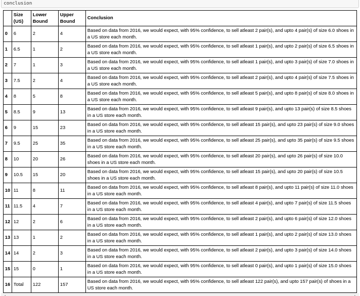

可能進一步分析 (Possibly Further Analysis)

The same analysis above can all be completed for different 'Gender', 'Country' and 'Year' values. In total this would produce 2 x 4 x 3 = 24 different sets of bounds to guide the retailer. These bounds could be used to guide a retailer in each specific circumstance. Alternatively, if these results don't differ much we may use this as a reason to use a larger data set. For example, if our bounds don't change much for each 'Year', we may want to use the 'Male' 'United States' data from all years to get a more accurate result.

對于不同的'Gender' ， 'Country'和'Year'值，都可以完成以上相同的分析。 總體而言，這將產生2 x 4 x 3 = 24組不同的邊界以指導零售商。 這些界限可以用來指導零售商在每種特定情況下。 另外，如果這些結果相差不大，我們可以以此為理由使用較大的數據集。 例如，如果每個'Year'界限變化不大，我們可能希望使用所有年份的'Male' 'United States'數據來獲得更準確的結果。

Thanks for reading and thanks to Nhan Tran for the original post that guided this project.

感謝您的閱讀，也感謝Nhan Tran提供了指導該項目的原始文章。

The code for this project can be found at my GitHub.

該項目的代碼可以在我的GitHub上找到 。