現實世界中的數據科學 (Data Science in the Real World)

This article aims to present two ways of calculating non linear correlation between any number of discrete variables. The objective for a data analysis project is twofold : on the one hand, to know the amount of information the variables share with each other, and therefore, to identify whether the data available contain the information one is looking for ; and on the other hand, to identify which minimum set of variables contains the most important amount of useful information.

本文旨在介紹兩種計算任意數量的離散變量之間的非線性相關性的方法。 數據分析項目的目標是雙重的：一方面，了解變量之間共享的信息量，從而確定可用數據是否包含人們正在尋找的信息； 另一方面，確定哪些最小變量集包含最重要的有用信息量。

變量之間的不同類型的關系 (The different types of relationships between variables)

線性度 (Linearity)

The best-known relationship between several variables is the linear one. This is the type of relationships that is measured by the classical correlation coefficient: the closer it is, in absolute value, to 1, the more the variables are linked by an exact linear relationship.

幾個變量之間最著名的關系是線性關系。 這是用經典相關系數衡量的關系類型：絕對值越接近1，變量之間通過精確的線性關系鏈接的越多。

However, there are plenty of other potential relationships between variables, which cannot be captured by the measurement of conventional linear correlation.

但是，變量之間還有許多其他潛在的關系，無法通過常規線性相關性的測量來捕獲。

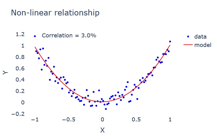
To find such non-linear relationships between variables, other correlation measures should be used. The price to pay is to work only with discrete, or discretized, variables.

為了找到變量之間的這種非線性關系，應該使用其他相關度量。 要付出的代價是僅對離散變量或離散變量起作用。

In addition to that, having a method for calculating multivariate correlations makes it possible to take into account the two main types of interaction that variables may present: relationships of information redundancy or complementarity.

除此之外，擁有一種用于計算多元相關性的方法，可以考慮變量可能呈現的兩種主要交互類型：信息冗余或互補性的關系。

冗余 (Redundancy)

When two variables (hereafter, X and Y) share information in a redundant manner, the amount of information provided by both variables X and Y to predict Z will be inferior to the sum of the amounts of information provided by X to predict Z, and by Y to predict Z.

當兩個變量(以下，X和Y)以冗余的方式共享信息，由兩個變量X和Y中提供的信息來預測的Z量將不如由X所提供的預測的Z信息的量的總和，和由Y預測Z。

In the extreme case, X = Y. Then, if the values taken by Z can be correctly predicted 50% of the times by X (and Y), the values taken by Z cannot be predicted perfectly (i.e. 100% of the times) by the variables X and Y together.

在極端情況下， X = Y。 然后，如果可以通過X (和Y )正確地預測Z所取的值的50％時間，則變量X和Y不能一起完美地預測Z所取的值(即100％的時間)。

                            ╔═══╦═══╦═══╗
                            ║ X ║ Y ║ Z ║
                            ╠═══╬═══╬═══╣
                            ║ 0 ║ 0 ║ 0 ║
                            ║ 0 ║ 0 ║ 0 ║
                            ║ 1 ║ 1 ║ 0 ║
                            ║ 1 ║ 1 ║ 1 ║
                            ╚═══╩═══╩═══╝

互補性 (Complementarity)

The complementarity relationship is the exact opposite situation. In the extreme case, X provides no information about Z, neither does Y, but the variables X and Y together allow to predict perfectly the values taken by Z. In such a case, the correlation between X and Z is zero, as is the correlation between Y and Z, but the correlation between X, Y and Z is 100%.

互補關系是完全相反的情況。 在極端情況下， X不提供有關Z的信息， Y也不提供任何信息，但是變量X和Y一起可以完美地預測Z所取的值。 在這種情況下， X和Z之間的相關性為零， Y和Z之間的相關性也為零，但是X ， Y和Z之間的相關性為100％。

These complementarity relationships only occur in the case of non-linear relationships, and must then be taken into account in order to avoid any error when trying to reduce the dimensionality of a data analysis problem: discarding X and Y because they do not provide any information on Z when considered independently would be a bad idea.

這些互補關系僅在非線性關系的情況下發生，然后在嘗試減小數據分析問題的維數時必須考慮到它們以避免錯誤：丟棄X和Y，因為它們不提供任何信息在Z上單獨考慮時，將是一個壞主意。

                            ╔═══╦═══╦═══╗
                            ║ X ║ Y ║ Z ║
                            ╠═══╬═══╬═══╣
                            ║ 0 ║ 0 ║ 0 ║
                            ║ 0 ║ 1 ║ 1 ║
                            ║ 1 ║ 0 ║ 1 ║
                            ║ 1 ║ 1 ║ 0 ║
                            ╚═══╩═══╩═══╝

“多元非線性相關性”的兩種可能測度 (Two possible measures of “multivariate non-linear correlation”)

There is a significant amount of possible measures of (multivariate) non-linear correlation (e.g. multivariate mutual information, maximum information coefficient — MIC, etc.). I present here two of them whose properties, in my opinion, satisfy exactly what one would expect from such measures. The only caveat is that they require discrete variables, and are very computationally intensive.

存在(多元)非線性相關性的大量可能度量(例如多元互信息，最大信息系數MIC等)。 我在這里介紹他們中的兩個，我認為它們的性質完全滿足人們對此類措施的期望。 唯一的警告是它們需要離散變量，并且計算量很大。

對稱測度 (Symmetric measure)

The first one is a measure of the information shared by n variables V1, …, Vn, known as “dual total correlation” (among other names).

第一個是對n個變量V1，…，Vn共享的信息的度量，稱為“雙重總相關”(在其他名稱中)。

This measure of the information shared by different variables can be characterized as:

不同變量共享的信息的這種度量可以表征為：

where H(V) expresses the entropy of variable V.

其中H(V)表示變量V的熵。

When normalized by H(V1, …, Vn), this “mutual information score” takes values ranging from 0% (meaning that the n variables are not at all similar) to 100% (meaning that the n variables are identical, except for the labels).

當用H(V1，…，Vn)歸一化時，該“互信息分”取值范圍從0％(意味著n個變量根本不相似)到100％(意味著n個變量相同，除了標簽)。

This measure is symmetric because the information shared by X and Y is exactly the same as the information shared by Y and X.

此度量是對稱的，因為X和Y共享的信息與Y和X共享的信息完全相同。

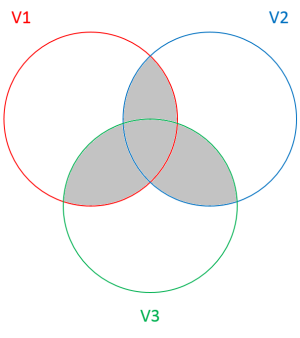
The Venn diagram above shows the “variability” (entropy) of the variables V1, V2 and V3 with circles. The shaded area represents the entropy shared by the three variables: it is the dual total correlation.

上方的維恩圖用圓圈顯示變量V1 ， V2和V3的“變異性”(熵)。 陰影區域表示三個變量共享的熵：它是對偶總相關。

不對稱測度 (Asymmetric measure)

The symmetry property of usual correlation measurements is sometimes criticized. Indeed, if I want to predict Y as a function of X, I do not care if X and Y have little information in common: all I care about is that the variable X contains all the information needed to predict Y, even if Y gives very little information about X. For example, if X takes animal species and Y takes animal families as values, then X easily allows us to know Y, but Y gives little information about X:

常用的相關測量的對稱性有時會受到批評。 的確，如果我想將Y預測為X的函數，則我不在乎X和Y是否有很少的共同點信息：我只關心變量X包含預測Y所需的所有信息，即使Y給出關于X的信息很少。 例如，如果X取動物種類而Y取動物種類作為值，則X容易使我們知道Y ，但Y幾乎沒有提供有關X的信息：

    ╔═════════════════════════════╦══════════════════════════════╗
    ║ Animal species (variable X) ║ Animal families (variable Y) ║
    ╠═════════════════════════════╬══════════════════════════════╣
    ║ Tiger                       ║ Feline                       ║
    ║ Lynx                        ║ Feline                       ║
    ║ Serval                      ║ Feline                       ║
    ║ Cat                         ║ Feline                       ║
    ║ Jackal                      ║ Canid                        ║
    ║ Dhole                       ║ Canid                        ║
    ║ Wild dog                    ║ Canid                        ║
    ║ Dog                         ║ Canid                        ║
    ╚═════════════════════════════╩══════════════════════════════╝

The “information score” of X to predict Y should then be 100%, while the “information score” of Y for predicting X will be, for example, only 10%.

那么，用于預測Y的X的“信息分數”應為100％，而用于預測X的Y的“信息分數”僅為例如10％。

In plain terms, if the variables D1, …, Dn are descriptors, and the variables T1, …, Tn are target variables (to be predicted by descriptors), then such an information score is given by the following formula:

簡而言之，如果變量D1，...，Dn是描述符，變量T1，...，Tn是目標變量(將由描述符預測)，則這樣的信息得分將由以下公式給出：

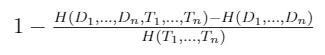
where H(V) expresses the entropy of variable V.

其中H(V)表示變量V的熵。

This “prediction score” also ranges from 0% (if the descriptors do not predict the target variables) to 100% (if the descriptors perfectly predict the target variables). This score is, to my knowledge, completely new.

此“預測分數”的范圍也從0％(如果描述符未預測目標變量)到100％(如果描述符完美地預測目標變量)。 據我所知，這個分數是全新的。

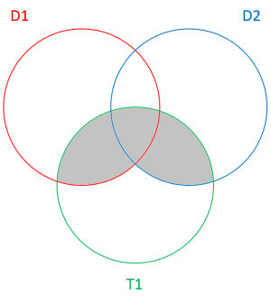
The shaded area in the above diagram represents the entropy shared by the descriptors D1 and D2 with the target variable T1. The difference with the dual total correlation is that the information shared by the descriptors but not related to the target variable is not taken into account.

上圖中的陰影區域表示描述符D1和D2與目標變量T1共享的熵。 與雙重總相關的區別在于，不考慮描述符共享但與目標變量無關的信息。

實際中信息分數的計算 (Computation of the information scores in practice)

A direct method to calculate the two scores presented above is based on the estimation of the entropies of the different variables, or groups of variables.

計算上述兩個分數的直接方法是基于對不同變量或變量組的熵的估計。

In R language, the entropy function of the ‘infotheo’ package gives us exactly what we need. The calculation of the joint entropy of three variables V1, V2 and V3 is very simple:

在R語言中，“ infotheo”程序包的熵函數提供了我們所需的信息。 三個變量V1 ， V2和V3的聯合熵的計算非常簡單：

library(infotheo)df <- data.frame(V1 = c(0,0,1,1,0,0,1,0,1,1),                 V2 = c(0,1,0,1,0,1,1,0,1,0),                 V3 = c(0,1,1,0,0,0,1,1,0,1))entropy(df)[1] 1.886697

The computation of the joint entropy of several variables in Python requires some additional work. The BIOLAB contributor, on the blog of the Orange software, suggests the following function:

Python中幾個變量的聯合熵的計算需要一些額外的工作。 BIOLAB貢獻者在Orange軟件的博客上建議了以下功能：

import numpy as np
import itertools
from functools import reducedef entropy(*X):    entropy = sum(-p * np.log(p) if p > 0 else 0 for p in
        (np.mean(reduce(np.logical_and, (predictions == c for predictions, c in zip(X, classes))))
        for classes in itertools.product(*[set(x) for x in X])))    return(entropy)V1 = np.array([0,0,1,1,0,0,1,0,1,1])V2 = np.array([0,1,0,1,0,1,1,0,1,0])V3 = np.array([0,1,1,0,0,0,1,1,0,1])entropy(V1, V2, V3)1.8866967846580784

In each case, the entropy is given in nats, the “natural unit of information”.

在每種情況下，熵都以nat(“信息的自然單位”)給出。

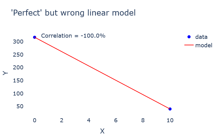
For a high number of dimensions, the information scores are no longer computable, as the entropy calculation is too computationally intensive and time-consuming. Also, it is not desirable to calculate information scores when the number of samples is not large enough compared to the number of dimensions, because then the information score is “overfitting” the data, just like in a classical machine learning model. For instance, if only two samples are available for two variables X and Y, the linear regression will obtain a “perfect” result:

對于大量維，信息分數不再可計算，因為熵計算的計算量很大且很耗時。 同樣，當樣本數量與維數相比不夠大時，也不希望計算信息分數，因為就像經典的機器學習模型一樣，信息分數會使數據“過度擬合”。 例如，如果對于兩個變量X和Y只有兩個樣本可用，則線性回歸將獲得“完美”的結果：

                            ╔════╦═════╗
                            ║ X  ║  Y  ║
                            ╠════╬═════╣
                            ║  0 ║ 317 ║
                            ║ 10 ║  40 ║
                            ╚════╩═════╝

Similarly, let’s imagine that I take temperature measures over time, while ensuring to note the time of day for each measure. I can then try to explore the relationship between time of day and temperature. If the number of samples I have is too small relative to the number of problem dimensions, the chances are high that the information scores overestimate the relationship between the two variables:

同樣，讓我們??想象一下，我會隨著時間的推移進行溫度測量，同時確保記下每個測量的時間。 然后，我可以嘗試探索一天中的時間與溫度之間的關系。 如果我擁有的樣本數量相對于問題維度的數量而言太少，則信息分數很有可能高估了兩個變量之間的關系：

                ╔══════════════════╦════════════════╗
                ║ Temperature (°C) ║ Hour (0 to 24) ║
                ╠══════════════════╬════════════════╣
                ║               23 ║             10 ║
                ║               27 ║             15 ║
                ╚══════════════════╩════════════════╝

In the above example, and based on the only observations available, it appears that the two variables are in perfect bijection: the information scores will be 100%.

在上面的示例中，并且基于僅可用的觀察結果，看來這兩個變量完全是雙射的：信息得分將為100％。

It should therefore be remembered that information scores are capable, like machine learning models, of “overfitting”, much more than linear correlation, since linear models are by nature limited in complexity.

因此，應該記住，信息評分像機器學習模型一樣，具有“過擬合”的能力，遠遠超過了線性相關性，因為線性模型天生就受到復雜性的限制。

預測分數使用示例 (Example of prediction score use)

The Titanic dataset contains information about 887 passengers from the Titanic who were on board when the ship collided with an iceberg: the price they paid for boarding (Fare), their class (Pclass), their name (Name), their gender (Sex), their age (Age), the number of their relatives on board (Parents/Children Aboard and Siblings/Spouses Aboard) and whether they survived or not (Survived).

泰坦尼克號數據集包含有關當泰坦尼克號與冰山相撞時在船上的887名乘客的信息：他們所支付的登船價格( 車費 )，其艙位( Pclass )，姓名( Name )，性別( Sex ) ，他們的年齡( Age )，在船上的親戚數( 父母/子女和兄弟姐妹/配偶 )以及他們是否幸存( Survived )。

This dataset is typically used to determine the probability that a person had of surviving, or more simply to “predict” whether the person survived, by means of the individual data available (excluding the Survived variable).

該數據集通常用于通過可用的個人數據(不包括生存變量)來確定一個人生存的可能性，或更簡單地“預測”該人是否生存 。

So, for different possible combinations of the descriptors, I calculated the prediction score with respect to the Survived variable. I removed the nominative data (otherwise the prediction score would be 100% because of the overfitting) and discretized the continuous variables. Some results are presented below:

因此，對于描述符的不同可能組合，我針對生存變量計算了預測得分。 我刪除了名義數據(否則，由于過度擬合，預測得分將為100％)，并離散化了連續變量。 一些結果如下所示：

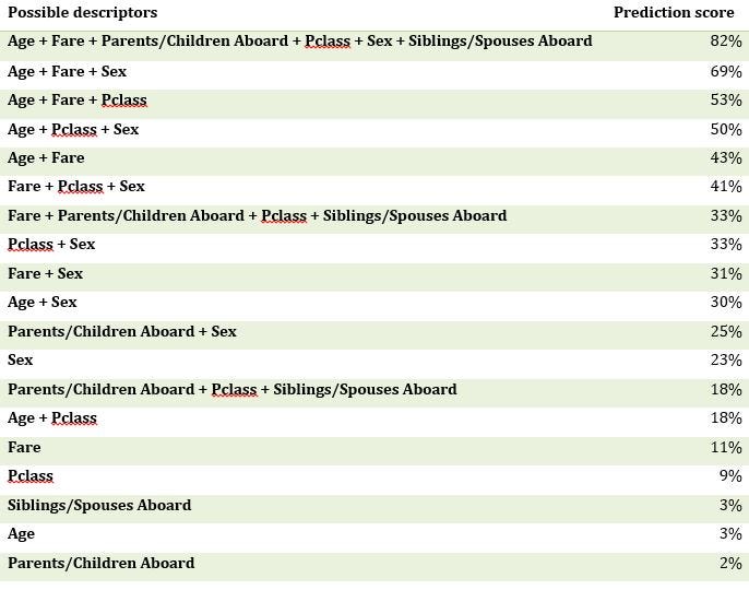
The first row of the table gives the prediction score if we use all the predictors to predict the target variable: this score being more than 80%, it is clear that the available data enable us to predict with a “good precision” the target variable Survived.

如果我們使用所有預測變量來預測目標變量，則表的第一行將給出預測得分：該得分超過80％，很明顯，可用數據使我們能夠“精確”地預測目標變量幸存下來 。

Cases of information redundancy can also be observed: the variables Fare, PClass and Sex are together correlated at 41% with the Survived variable, while the sum of the individual correlations amounts to 43% (11% + 9% + 23%).

信息冗余的情況下，也可以觀察到：變量票價 ，PClass和性別在與幸存變量41％一起相關，而各個相關性的總和達43％(11％+ 9％+ 23％)。

There are also cases of complementarity: the variables Age, Fare and Sex are almost 70% correlated with the Survived variable, while the sum of their individual correlations is not even 40% (3% + 11% + 23%).

還有互補的情況： 年齡 ， 票價和性別變量與生存變量幾乎有70％相關，而它們各自的相關總和甚至不到40％(3％+ 11％+ 23％)。

Finally, if one wishes to reduce the dimensionality of the problem and to find a “sufficiently good” model using as few variables as possible, it is better to use the three variables Age and Fare and Sex (prediction score of 69%) rather than the variables Fare, Parents/Children Aboard, Pclass and Siblings/Spouses Aboard (prediction score of 33%). It allows to find twice as much useful information with one less variable.

最后，如果希望減少問題的范圍并使用盡可能少的變量來找到“足夠好”的模型，則最好使用年齡 ， 票價和性別這三個變量(預測得分為69％)，而不是變量票價 ， 家長 / 兒童 到齊 ，Pclass和兄弟姐妹 / 配偶 到齊 (33％預測得分)。 它允許查找變量少一倍的有用信息。

Calculating the prediction score can therefore be very useful in a data analysis project, to ensure that the data available contain sufficient relevant information, and to identify the variables that are most important for the analysis.

因此，在數據分析項目中，計算預測分數可能非常有用，以確保可用數據包含足夠的相關信息，并確定對于分析最重要的變量。