Multivariate Time Series Analysis

多元時間序列分析

A univariate time series data contains only one single time-dependent variable while a multivariate time series data consists of multiple time-dependent variables. We generally use multivariate time series analysis to model and explain the interesting interdependencies and co-movements among the variables. In the multivariate analysis — the assumption is that the time-dependent variables not only depend on their past values but also show dependency between them. Multivariate time series models leverage the dependencies to provide more reliable and accurate forecasts for a specific given data, though the univariate analysis outperforms multivariate in general[1]. In this article, we apply a multivariate time series method, called Vector Auto Regression (VAR) on a real-world dataset.

單變量時間序列數據僅包含一個時間相關的變量，而多元時間序列數據則包含多個時間相關的變量。 我們通常使用多元時間序列分析來建模和解釋變量之間有趣的相互依存關系和共同運動。 在多變量分析中，假定時間相關變量不僅取決于它們的過去值，而且還顯示它們之間的依賴關系。 多元時間序列模型利用依存關系為特定的給定數據提供更可靠，更準確的預測，盡管單變量分析通常優于多元變量[1]。 在本文中，我們在現實世界的數據集上應用了一種稱為向量自動回歸(VAR)的多元時間序列方法。

Vector Auto Regression (VAR)

向量自回歸(VAR)

VAR model is a stochastic process that represents a group of time-dependent variables as a linear function of their own past values and the past values of all the other variables in the group.

VAR模型是一個隨機過程，將一組時間相關變量表示為它們自己的過去值以及該組中所有其他變量的過去值的線性函數。

For instance, we can consider a bivariate time series analysis that describes a relationship between hourly temperature and wind speed as a function of past values [2]:

例如，我們可以考慮一個雙變量時間序列分析，該分析描述了每小時溫度和風速之間的關系，該關系是過去值的函數[2]：

temp(t) = a1 + w11* temp(t-1) + w12* wind(t-1) + e1(t-1)

temp(t)= a1 + w11 * temp(t-1)+ w12 * wind(t-1)+ e1(t-1)

wind(t) = a2 + w21* temp(t-1) + w22*wind(t-1) +e2(t-1)

wind(t)= a2 + w21 * temp(t-1)+ w22 * wind(t-1)+ e2(t-1)

where a1 and a2 are constants; w11, w12, w21, and w22 are the coefficients; e1 and e2 are the error terms.

其中a1和a2是常數； w11，w12，w21和w22是系數； e1和e2是誤差項。

Dataset

數據集

Statmodels is a python API that allows users to explore data, estimate statistical models, and perform statistical tests [3]. It contains time series data as well. We download a dataset from the API.

Statmodels是python API，允許用戶瀏覽數據，估計統計模型并執行統計測試[3]。 它還包含時間序列數據。 我們從API下載數據集。

To download the data, we have to install some libraries and then load the data:

要下載數據，我們必須安裝一些庫，然后加載數據：

import pandas as pd
import statsmodels.api as sm
from statsmodels.tsa.api import VAR
data = sm.datasets.macrodata.load_pandas().data
data.head(2)

The output shows the first two observations of the total dataset:

輸出顯示了總數據集的前兩個觀察值：

The data contains a number of time-series data, we take only two time-dependent variables “realgdp” and “realdpi” for experiment purposes and use “year” columns as the index of the data.

數據包含許多時間序列數據，出于實驗目的，我們僅采用兩個與時間相關的變量“ realgdp”和“ realdpi”，并使用“ year”列作為數據索引。

data1 = data[["realgdp", 'realdpi']]
data1.index = data["year"]

output:

輸出：

Let's visualize the data:

讓我們可視化數據：

data1.plot(figsize = (8,5))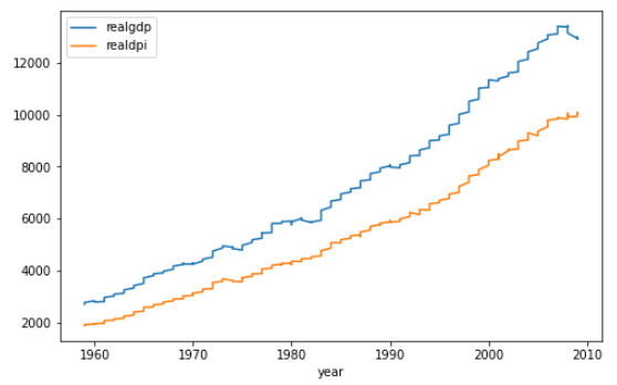

Both of the series show an increasing trend over time with slight ups and downs.

這兩個系列都顯示出隨著時間的推移呈上升趨勢，并有輕微的起伏。

Stationary

固定式

Before applying VAR, both the time series variable should be stationary. Both the series are not stationary since both the series do not show constant mean and variance over time. We can also perform a statistical test like the Augmented Dickey-Fuller test (ADF) to find stationarity of the series using the AIC criteria.

應用VAR之前，兩個時間序列變量均應為固定值。 兩個序列都不是平穩的，因為兩個序列都沒有顯示出恒定的均值和隨時間變化。 我們還可以執行統計測試(如增強迪基-富勒檢驗(ADF))，以使用AIC標準查找系列的平穩性。

adfuller_test = adfuller(data1['realgdp'], autolag= "AIC")
print("ADF test statistic: {}".format(adfuller_test[0]))
print("p-value: {}".format(adfuller_test[1]))

output:

輸出：

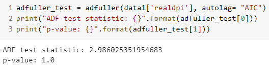
In both cases, the p-value is not significant enough, meaning that we can not reject the null hypothesis and conclude that the series are non-stationary.

在這兩種情況下，p值都不足夠顯著，這意味著我們不能拒絕原假設并得出結論該序列是非平穩的。

Differencing

差異化

As both the series are not stationary, we perform differencing and later check the stationarity.

由于兩個系列都不平穩，因此我們進行微分，然后檢查平穩性。

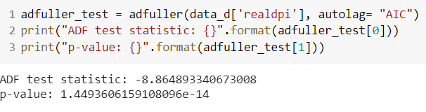
data_d = data1.diff().dropna()

The “realgdp” series becomes stationary after first differencing of the original series as the p-value of the test is statistically significant.

由于測試的p值具有統計意義，因此“ realgdp”系列在對原始系列進行第一次求差后將變得平穩。

The “realdpi” series becomes stationary after first differencing of the original series as the p-value of the test is statistically significant.

由于原始的p值在統計上具有顯著性，因此“ realdpi”系列在與原始系列進行首次差異化處理后就變得穩定了。

Model

模型

In this section, we apply the VAR model on the one differenced series. We carry-out the train-test split of the data and keep the last 10-days as test data.

在本節中，我們將VAR模型應用于一個差分序列。 我們對數據進行火車測試拆分，并保留最后10天作為測試數據。

train = data_d.iloc[:-10,:]
test = data_d.iloc[-10:,:]

Searching optimal order of VAR model

搜索VAR模型的最優階

In the process of VAR modeling, we opt to employ Information Criterion Akaike (AIC) as a model selection criterion to conduct optimal model identification. In simple terms, we select the order (p) of VAR based on the best AIC score. The AIC, in general, penalizes models for being too complex, though the complex models may perform slightly better on some other model selection criterion. Hence, we expect an inflection point in searching the order (p), meaning that, the AIC score should decrease with order (p) gets larger until a certain order and then the score starts increasing. For this, we perform grid-search to investigate the optimal order (p).

在VAR建模過程中，我們選擇采用信息準則赤池(AIC)作為模型選擇標準來進行最佳模型識別。 簡單來說，我們根據最佳AIC得分選擇VAR的階數(p)。 通常，AIC會因過于復雜而對模型進行懲罰，盡管復雜模型在某些其他模型選擇標準上可能會稍好一些。 因此，我們期望在搜索階數(p)時出現拐點，這意味著，隨著階數(p)的增大，AIC分數應減小，直到達到某個階數，然后分數才開始增加。 為此，我們執行網格搜索以研究最佳階數(p)。

forecasting_model = VAR(train)results_aic = []
for p in range(1,10):
  results = forecasting_model.fit(p)
  results_aic.append(results.aic)

In the first line of the code: we train VAR model with the training data. Rest of code: perform a for loop to find the AIC scores for fitting order ranging from 1 to 10. We can visualize the results (AIC scores against orders) to better understand the inflection point:

在代碼的第一行：我們使用訓練數據訓練VAR模型。 其余代碼：執行for循環以找到適合訂單的AIC得分，范圍從1到10。我們可以可視化結果(針對訂單的AIC得分)，以更好地了解拐點：

import seaborn as sns
sns.set()
plt.plot(list(np.arange(1,10,1)), results_aic)
plt.xlabel("Order")
plt.ylabel("AIC")
plt.show()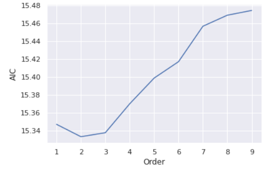

From the plot, the lowest AIC score is achieved at the order of 2 and then the AIC scores show an increasing trend with the order p gets larger. Hence, we select the 2 as the optimal order of the VAR model. Consequently, we fit order 2 to the forecasting model.

從圖中可以看到，最低的AIC得分約為2，然后，隨著p的增大，AIC得分呈上升趨勢。 因此，我們選擇2作為VAR模型的最優順序。 因此，我們將訂單2擬合到預測模型。

let's check the summary of the model:

讓我們檢查一下模型的摘要：

results = forecasting_model.fit(2)
results.summary()

The summary output contains much information:

摘要輸出包含許多信息：

Forecasting

預測

We use 2 as the optimal order in fitting the VAR model. Thus, we take the final 2 steps in the training data for forecasting the immediate next step (i.e., the first day of the test data).

我們使用2作為擬合VAR模型的最佳順序。 因此，我們在訓練數據中采取最后的2個步驟來預測下一步(即測試數據的第一天)。

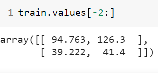
Now, after fitting the model, we forecast for the test data where the last 2 days of training data set as lagged values and steps set as 10 days as we want to forecast for the next 10 days.

現在，在擬合模型之后，我們預測測試數據，其中訓練數據的最后2天設置為滯后值，步長設置為10天，因為我們希望在接下來的10天進行預測。

laaged_values = train.values[-2:]forecast = pd.DataFrame(results.forecast(y= laaged_values, steps=10), index = test.index, columns= ['realgdp_1d', 'realdpi_1d'])forecast

The output:

輸出：

We have to note that the aforementioned forecasts are for the one differenced model. Hence, we must reverse the first differenced forecasts into the original forecast values.

我們必須注意，上述預測是針對一種差異模型的。 因此，我們必須將最初的差異預測反轉為原始預測值。

forecast["realgdp_forecasted"] = data1["realgdp"].iloc[-10-1] +   forecast_1D['realgdp_1d'].cumsum()forecast["realdpi_forecasted"] = data1["realdpi"].iloc[-10-1] +      forecast_1D['realdpi_1d'].cumsum() 

output:

輸出：

The first two columns are the forecasted values for 1 differenced series and the last two columns show the forecasted values for the original series.

前兩列是1個差異序列的預測值，后兩列顯示原始序列的預測值。

Now, we visualize the original test values and the forecasted values by VAR.

現在，我們通過VAR可視化原始測試值和預測值。

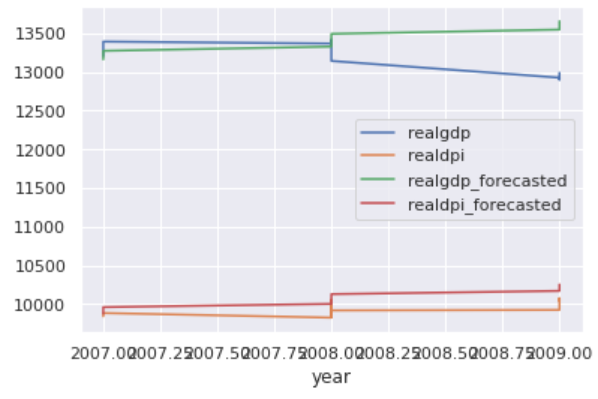
The original realdpi and the forecasted realdpi show a similar pattern throwout the forecasted days. For realgdp: the first half of the forecasted values show a similar pattern as the original values, on the other hand, the last half of the forecasted values do not follow similar pattern.

原始的realdpi和預測的realdpi顯示出相似的模式，從而排除了預測的天數。 對于realgdp：預測值的前半部分顯示與原始值相似的模式，另一方面，預測值的后半部分沒有遵循相似的模式。

To sum up, in this article, we discuss multivariate time series analysis and applied the VAR model on a real-world multivariate time series dataset.

綜上所述，在本文??中，我們討論了多元時間序列分析，并將VAR模型應用于實際的多元時間序列數據集。

You can also read the article — A real-world time series data analysis and forecasting, where I applied ARIMA (univariate time series analysis model) to forecast univariate time series data.

您還可以閱讀這篇文章- 真實的時間序列數據分析和預測 ，在這里我應用了ARIMA(單變量時間序列分析模型)來預測單變量時間序列數據。

[1] https://homepage.univie.ac.at/robert.kunst/prognos4.pdf

[1] https://homepage.univie.ac.at/robert.kunst/prognos4.pdf

[2] https://www.aptech.com/blog/introduction-to-the-fundamentals-of-time-series-data-and-analysis/

[2] https://www.aptech.com/blog/introduction-to-the-fundamentals-of-time-series-data-and-analysis/

[3] https://www.statsmodels.org/stable/index.html

[3] https://www.statsmodels.org/stable/index.html