If you are reading this, then you probably tried to predict who will survive the Titanic shipwreck. This Kaggle competition is a canonical example of machine learning, and a right of passage for any aspiring data scientist. What if instead of predicting who will survive, you only had to predict how many will survive? Or, what if you had to predict the average age of survivors, or the sum of the fare that the survivors paid?

如果您正在閱讀本文，那么您可能試圖預測誰將在泰坦尼克號沉船中幸存。 這場Kaggle競賽是機器學習的典范，也是任何有抱負的數據科學家的通行權。 如果不必預測誰將生存，而只需要預測多少將生存怎么辦？ 或者，如果您必須預測幸存者的平均年齡或幸存者支付的車費之和怎么辦？

There are many applications where classification predictions need to be aggregated. For example, a customer churn model may generate probabilities that a customer will churn, but the business may be interested in how many customers are predicted to churn, or how much revenue will be lost. Similarly, a model may give a probability that a flight will be delayed, but we may want to know how many flights will be delayed, or how many passengers are affected. Hong (2013) lists a number of other examples from actuarial assessment to warranty claims.

在許多應用中，需要匯總分類預測。 例如，客戶流失模型可能會產生客戶流失的概率，但是企業可能會對預計有多少客戶流失或將損失多少收入感興趣。 同樣，模型可能會給您一個航班延誤的可能性，但我們可能想知道有多少航班會延誤，或者有多少乘客受到影響。 Hong(2013)列舉了從精算評估到保修索賠的許多其他示例。

Most binary classification algorithms estimate probabilities that examples belong to the positive class. If we treat these probabilities as known values (rather than estimates), then the number of positive cases is a random variable with a Poisson Binomial probability distribution. (If the probabilities were all the same, the distribution would be Binomial.) Similarly, the sum of two-value random variables where one value is zero and the other value some other number (e.g. age, revenue) is distributed as a Generalized Poisson Binomial. Under these assumptions we can report mean values as well as prediction intervals. In summary, if we had the true classification probabilities, then we could construct the probability distributions of any aggregate outcome (number of survivors, age, revenue, etc.).

大多數二進制分類算法都會估計示例屬于肯定類的概率。 如果我們將這些概率視為已知值(而不是估計值)，則陽性病例數是具有泊松二項式概率分布的隨機變量。 (如果概率都相同，則分布將為二項式。)類似地，二值隨機變量的總和(其中一個值為零，而另一個值為其他數字(例如年齡，收入))作為廣義泊松分布二項式 在這些假設下，我們可以報告平均值以及預測間隔。 總而言之，如果我們擁有真正的分類概率，那么我們可以構建任何總體結果(幸存者的數量，年齡，收入等)的概率分布。

Of course, the classification probabilities we obtain from machine learning models are just estimates. Therefore, treating the probabilities as known values may not be appropriate. (Essentially, we would be ignoring the sampling error in estimating these probabilities.) However, if we are interested only in the aggregate characteristics of survivors, perhaps we should focus on estimating parameters that describe the probability distributions of these aggregate characteristics. In other words, we should recognize that we have a numerical prediction problem rather than a classification problem.

當然，我們從機器學習模型中獲得的分類概率只是估計值。 因此，將概率視為已知值可能不合適。 (從本質上講，在估計這些概率時，我們將忽略采樣誤差。)但是，如果我們僅對幸存者的總體特征感興趣，那么也許我們應該專注于估算描述這些總體特征的概率分布的參數。 換句話說，我們應該認識到我們有一個數值預測問題，而不是分類問題。

I compare two approaches to getting aggregate characteristics of Titanic survivors. The first is to classify and then aggregate. I estimate three popular classification models and then aggregate the resulting probabilities. The second approach is a regression model to estimate how aggregate characteristics of a group of passengers affect the share that survives. I evaluate each approach using many random splits of test and train data. The conclusion is that many classification models do poorly when the classification probabilities are aggregated.

我比較了兩種獲取泰坦尼克號幸存者總體特征的方法。 首先是分類，然后匯總 。 我估計了三種流行的分類模型，然后合計了得出的概率。 第二種方法是一種回歸模型，用于估計一組乘客的總體特征如何影響幸存的份額。 我使用許多隨機的測試和訓練數據評估每種方法。 結論是，當匯總分類概率時，許多分類模型的效果不佳。

1.分類和匯總方法 (1. Classify and Aggregate Approach)

Let’s use the Titanic data to estimate three different classifiers. The logistic model will use only age and passenger class as predictors; Random Forest and XGBoost will also use sex. I train the model on the 891 passengers in Kaggle’s training data. I evaluate the predictions on the 418 in the test data. (I obtained the labels for the test set to be able to evaluate my models.)

讓我們使用Titanic數據來估計三個不同的分類器。 邏輯模型將僅使用年齡和乘客等級作為預測因子； 隨機森林和XGBoost也將使用性別。 我在Kaggle的訓練數據中為891名乘客訓練了模型。 我在測試數據中評估418的預測。 (我獲得了測試集的標簽，以便能夠評估我的模型。)

The logistic model with only age and passenger class as predictors has an AUC of 0.67. Random Forest and XGBoost that also use sex reach a very respectable AUC of around 0.8. Our task, however, is to predict how many passengers will survive. We can estimate this by adding up the probabilities that a passenger will survive. Interestingly, of the three classifiers, the logistic model was the closest to the actual number of survivors despite having the lowest AUC. It is also worth noting that a naive estimate based on the share of survivors in the training data did best of all.

僅以年齡和乘客等級為預測因子的邏輯模型的AUC為0.67。 同樣使用性行為的Random Forest和XGBoost的AUC達到了非常可觀的0.8。 但是，我們的任務是預測有多少乘客能夠幸存。 我們可以通過將乘客生存的概率相加來估計這一點。 有趣的是，在三個分類器中，邏輯模型盡管AUC最低，但與實際幸存者數量最接近。 還值得注意的是，基于幸存者在訓練數據中所占份額的天真估計最能說明問題。

Given the probabilities of survival for each passenger in the test set, the number of passengers that will survive is a random variable distributed Poisson Binomial. The mean of this random variable is the sum of the individual probabilities. The percentiles of this distribution can be obtained using the `poibin` R package developed by Hong (2013). A similar package for Python is under development. The percentiles can also be obtained through brute force by simulating 10,000 different sets of outcomes for the 418 passengers in the test set. The percentiles can be interpreted as prediction intervals telling us that the actual number of survivors will be within this interval with 95% probability.

給定測試集中每個乘客的生存概率，將生存的乘客數量是一個隨機變量分布的Poisson Binomial。 該隨機變量的平均值是各個概率的總和。 可以使用Hong(2013)開發的`poibin` R軟件包來獲得該分布的百分位數。 類似的Python包正在開發中。 通過為測試集中的418位乘客模擬10,000種不同的結果集，還可以通過蠻力獲得百分位數。 百分位可以解釋為預測間隔，告訴我們幸存者的實際數量將以95％的概率在此間隔內。

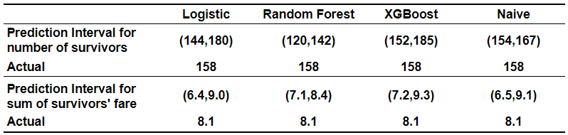
The interval based on the Random Forest probabilities widely missed the actual number of survivors. It is worth noting that the width of the interval is not necessarily based on the accuracy of the individual probabilities. Instead, it depends on how far those individual probabilities are from 0.5. Probabilities close to 0.9 or 0.1 rather than 0.5 mean that there is a lot less uncertainty as to how many passengers will survive. A good discussion of forecast reliability versus sharpness is here.

基于隨機森林概率的時間間隔大大錯過了幸存者的實際數量。 值得注意的是，間隔的寬度不一定基于各個概率的準確性。 取而代之的是，它取決于這些個體概率與0.5之間的差值。 概率接近0.9或0.1而不是0.5意味著，有多少乘客能夠幸存，其不確定性要小得多。 這里對預測的可靠性與清晰度進行了很好的討論。

While the number of survivors is a sum of zero/one random variables (Bernoulli trials), we may also be interested in predicting other aggregate characteristics of the survivors, e.g. total fare paid by the survivors. This measure is a sum of two-value random variables where one value is zero (passenger did not survive) and the other one is the fare that the passenger paid. Zhang, Hong and Balakrishnan (2018) call the probability distribution of this sum Generalized Poisson Binomial. As with Poisson Binomial, Hong, co-wrote an R package, GPB, that makes computing the probability distributions straightforward. Once again, simulating the distribution is an alternative to using the packages to compute percentiles.

雖然幸存者的數量是零/一個隨機變量的總和(Bernoulli試驗)，但我們也可能對預測幸存者的其他總體特征感興趣，例如，由幸存者支付的總票價。 此度量是兩個值隨機變量的總和，其中一個值為零(乘客無法幸存)，另一個為乘客支付的票價。 Zhang，Hong和Balakrishnan(2018)稱該和為廣義泊松二項式的概率分布。 像Hong的Poisson Binomial一樣，編寫了R程序包GPB ，這使得計算概率分布變得簡單。 再一次，模擬分布是使用軟件包計算百分位數的替代方法。

2.總體回歸法 (2. Aggregate Regression Approach)

If we only care about the aggregate characteristics of survivors, then we really have a numerical prediction problem. The simplest estimate of the share of survivors in the test set is the share of survivors in the training set — it is the naive estimate from the previous section. This estimate is probably unbiased and efficient if the characteristics of passengers in the test and train sets are identical. If not, then we would want an estimate of the share of survivors conditional on the characteristics of the passengers.

如果我們只關心幸存者的總體特征，那么我們確實有一個數值預測問題。 測試集中幸存者份額的最簡單估計是訓練集中幸存者的份額-這是上一節中的幼稚估計。 如果測試組和火車組中的乘客特征相同，則此估計可能是公正且有效的。 如果沒有，那么我們將希望根據乘客的特征估算幸存者的份額。

The issue is that we don’t have the data to estimate how aggregate characteristics of a group of passengers affect the share that survived. After all, the Titanic hit the iceberg only once. Perhaps in other applications such as customer churn, we may have new data every month.

問題在于，我們沒有數據來估計一組乘客的總體特征如何影響幸存的份額。 畢竟，泰坦尼克號只擊中了冰山一次。 也許在其他應用程序(例如客戶流失)中，我們可能每個月都有新數據。

In the Titanic case I resort to simulating many different training data sets by re-sampling the original training data set. I calculate the average characteristics of each simulated data set to estimate of how these characteristics affect the share that will survive. I then take the average characteristics of passengers in the test set and predict how many will survive in the test set. There are many different ways one could summarize the aggregate characteristics. I use the share of passengers in first class, the share of passengers under the age of 10 and the share of female passengers. Not surprisingly, the samples of passengers that have more women, children and first class passengers have a higher share of survivors.

在泰坦尼克號案例中，我通過對原始訓練數據集進行重新采樣來模擬許多不同的訓練數據集。 我計算每個模擬數據集的平均特征，以估計這些特征如何影響將生存的份額。 然后，我將測試集中的乘客的平均特征，并預測有多少人將在測試集中幸存。 有多種不同的方式可以總結總體特征。 我使用頭等艙乘客的份額，10歲以下乘客的份額和女性乘客的份額。 毫不奇怪，擁有更多婦女，兒童和頭等艙乘客的乘客樣本中幸存者的比例更高。

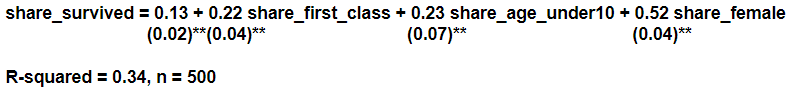
Applying the above equation to aggregate characteristics of the test data, I predict 162 survivors against the actual of 158 with a prediction interval of 151 to 173. Thus, the regression approach worked quite well.

將上述方程式應用到測試數據的總體特征中，我預測了162個幸存者，而實際值是158，而預測間隔為151到173。因此，回歸方法工作得很好。

3.兩種方法比較如何？ (3. How Do the Two Approaches Compare?)

So far, we evaluated the two approaches using only one test set. In order to compare the two approaches more systematically, I re-sampled from the union of the original train and test data set to create five hundred new train and test data sets. I then applied the two approaches five hundred times and calculated the mean square error of each approach across these five hundred samples. The graphs below show the relative performance of each approach.

到目前為止，我們僅使用一個測試集評估了這兩種方法。 為了更系統地比較這兩種方法，我從原始火車和測試數據集的聯合中重新采樣以創建五百個新的火車和測試數據集。 然后，我對這兩種方法進行了500次應用，并計算了這500種樣本中每種方法的均方誤差。 下圖顯示了每種方法的相對性能。

Among the classification models, the logistic model did best (had the lowest MSE). XGBoost is a relatively close second. Random Forest is way off. The accuracy of aggregate predictions depends crucially on the accuracy of the estimated probabilities. The logistic regression directly estimates the probability of survival. Similarly, XGBoost optimizes a logistic loss function. Therefore, both provide a decent estimate of probabilities. In contrast, Random Forest estimates probabilities as shares of trees that classified the example as success. As pointed out by Olson and Wyner (2018), the share of trees that classified the example as a success has nothing to do with the probability that the example will be a success. (For the same reason, calibration plots for Random Forest tend to be poor.) Although Random Forest can deliver a high AUC, the estimated probabilities are inappropriate for aggregation.

在分類模型中，邏輯模型表現最好(MSE最低)。 XGBoost相對來說排名第二。 隨機森林漸行漸遠。 聚合預測的準確性主要取決于估計概率的準確性。 邏輯回歸直接估計生存的可能性。 同樣，XGBoost優化了物流損失功能。 因此，兩者都提供了不錯的概率估計。 相反，隨機森林將概率估計為將示例歸類為成功的樹木份額。 正如Olson和Wyner(2018)指出的那樣，將示例成功分類為樹木的份額與示例成功的可能性無關。 (出于同樣的原因，隨機森林的標定圖往往很差。)盡管隨機森林可以提供較高的AUC，但估計的概率不適合匯總。

The aggregate regression model had the lowest MSE of all the approaches, beating even the classification logistic model. The naive predictions are handicapped in this evaluation because the share of survivors in the test data is not independent of the share of survivors in the train data. If we happen to have many survivors in the train, we will naturally have fewer survivors in the test. Even with this handicap, naive predictions handily beat XGBoost and Random Forest.

總體回歸模型具有所有方法中最低的MSE，甚至超過了分類邏輯模型。 由于測試數據中幸存者的比例與火車數據中幸存者的比例無關，因此天真的預測在此評估中受到了限制。 如果我們碰巧有很多幸存者在火車上，那么我們自然會減少測試中的幸存者。 即使有這種障礙，幼稚的預測也輕易擊敗了XGBoost和Random Forest。

4。結論 (4. Conclusion)

If we only need aggregate characteristics, estimating and aggregating individual classification probabilities seems like more trouble than is needed. In many cases, the share of survivors in the train set is a pretty good estimate of the share of survivors in the test set. Customer churn rate this month is probably a pretty good estimate of churn rate next month. More complicated models are worth building if we want to understand what drives survival or churn. It is also worth building more complicated models when our training data has very different characteristics than the test data, and when these characteristics affect survival or churn. Still, even in these cases, it is clear that using methods that are optimized for individual classifications could be inferior to methods optimized for a numerical prediction when a numerical prediction is needed.

如果我們只需要匯總特征，則估計和匯總單個分類概率似乎比需要的麻煩更多。 在許多情況下，訓練集中幸存者的比例是對測試集中幸存者比例的一個很好的估計。 本月的客戶流失率可能是下個月流失率的相當不錯的估計。 如果我們想了解驅動生存或流失的因素，則更復雜的模型值得構建。 當我們的訓練數據與測試數據具有非常不同的特征并且這些特征影響生存或流失時，也值得建立更復雜的模型。 盡管如此，即使在這些情況下，很明顯，當需要數值預測時，使用針對單個分類優化的方法可能不如針對數值預測優化的方法。

You can find the R code behind this note here.

您可以在此處找到此注釋后面的R代碼。