Article outline

文章大綱

• Introduction
  介紹
• Data Background
  資料背景
• Aim of the article
  本文的目的
• Exploratory analysis
  探索性分析
• Training a Random Forest Model
  訓練隨機森林模型
• Global Importance
  全球重要性
• Local Importance
  當地重要性

介紹 (Introduction)

In the supervised machine learning world, there are two types of algorithmic task often performed. One is called regression (predicting continuous values) and the other is called classification (predicting discrete values). Black box algorithms such as SVM, random forest, boosted trees, neural networks provide better prediction accuracy than conventional algorithms. The problem starts when we want to understand the impact (magnitude and direction) of different variables. In this article, I have presented an example of Random Forest binary classification algorithm and its interpretation at the global and local level using Local Interpretable Model-agnostic Explanations (LIME).

在有監督的機器學習世界中，經常執行兩種類型的算法任務。 一種稱為回歸(預測連續值)，另一種稱為分類(預測離散值)。 與傳統算法相比，諸如SVM，隨機森林，增強樹，神經網絡之類的黑匣子算法提供了更好的預測精度。 當我們想了解不同變量的影響(大小和方向)時，問題就開始了。 在本文中，我提供了一個使用本地可解釋模型不可知解釋(LIME)在全球和本地級別進行隨機森林二進制分類算法及其解釋的示例。

資料背景 (Data Background)

In this example, we are going to use the Pima Indian Diabetes 2 data set obtained from the UCI Repository of machine learning databases (Newman et al. 1998).

在本示例中，我們將使用從機器學習數據庫的UCI存儲庫中獲得的Pima Indian Diabetes 2數據集( Newman等，1998 )。

This data set is originally from the National Institute of Diabetes and Digestive and Kidney Diseases. The objective of the data set is to diagnostically predict whether or not a patient has diabetes, based on certain diagnostic measurements included in the data set. Several constraints were placed on the selection of these instances from a larger database. In particular, all patients here are females at least 21 years old of Pima Indian heritage.

該數據集最初來自美國國立糖尿病與消化與腎臟疾病研究所。 數據集的目的是根據數據集中包含的某些診斷測量值來診斷性預測患者是否患有糖尿病。 從較大的數據庫中選擇這些實例受到一些限制。 特別是，這里的所有患者均為皮馬印第安人血統至少21歲的女性。

The Pima Indian Diabetes 2 data set is the refined version (all missing values were assigned as NA) of the Pima Indian diabetes data. The data set contains the following independent and dependent variables.

Pima印度糖尿病2數據集是Pima印度糖尿病數據的精煉版本(所有缺失值均指定為NA)。 數據集包含以下獨立變量和因變量。

Independent variables (symbol: I)

自變量(符號：I)

• I1: pregnant: Number of times pregnant

  I1： 懷孕 ：懷孕次數

• I2: glucose: Plasma glucose concentration (glucose tolerance test)

  I2： 葡萄糖 ：血漿葡萄糖濃度(葡萄糖耐量試驗)

• I3: pressure: Diastolic blood pressure (mm Hg)

  I3： 壓力 ：舒張壓(毫米汞柱)

• I4: triceps: Triceps skin fold thickness (mm)

  I4： 三頭肌 ：三頭肌的皮膚折疊厚度(毫米)

• I5: insulin: 2-Hour serum insulin (mu U/ml)

  I5： 胰島素 ：2小時血清胰島素(mu U / ml)

• I6: mass: Body mass index (weight in kg/(height in m)\2)

  I6： 質量 ：體重指數(重量，單位：kg /(身高，單位：m)\2)

• I7: pedigree: Diabetes pedigree function

  I7： 譜系 ：糖尿病譜系功能

• I8: age: Age (years)

  I8： 年齡 ：年齡(年)

Dependent Variable (symbol: D)

因變量(符號：D)

• D1: diabetes: diabetes case (pos/neg)

  D1： 糖尿病 ：糖尿病病例(正/負)

建模目的 (Aim of the Modelling)

• fitting a random forest ensemble binary classification model that accurately predicts whether or not the patients in the data set have diabetes
  擬合隨機森林綜合二元分類模型，該模型可準確預測數據集中的患者是否患有糖尿病
• understanding the global influence of variables on diabetes prediction
  了解變量對糖尿病預測的全球影響
• understanding the influence of variables on the local level for the individual patient
  了解變量對個體患者局部水平的影響

加載庫 (Loading Libraries)

The very first step will be to load relevant libraries.

第一步將是加載相關的庫。

import pandas as pd             # data mnipulation
import numpy as np              # number manipulation/crunching
import matplotlib.pyplot as plt # plotting# Classification report
from sklearn.metrics import classification_report # Train Test split
from sklearn.model_selection import train_test_split# Random forest classifier
from sklearn.ensemble import RandomForestClassifier

Reading dataset

讀取數據集

After data loading, the next essential step is to perform an exploratory data analysis which helps in data familiarization. Use the head( ) function to view the top five rows of the data.

數據加載后，下一個基本步驟是執行探索性數據分析，這有助于數據熟悉。 使用head()函數查看數據的前五行。

diabetes = pd.read_csv("diabetes.csv")
diabetes.head()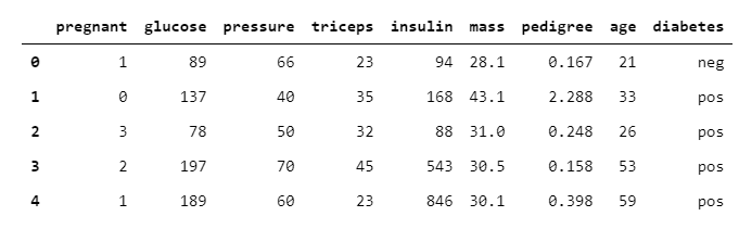

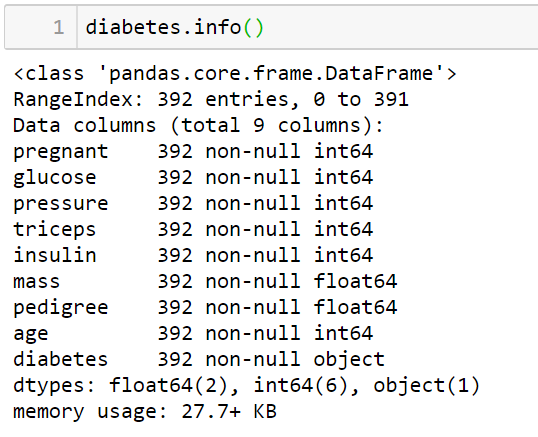
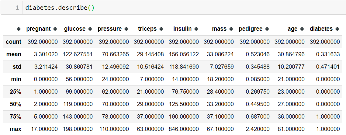
The below table showed that the diabetes data set includes 392 observations and 9 columns/variables. The independent variables include integer 64 and float 64 data types, whereas dependent/response (diabetes) variable is of string (neg/pos) data type also known as an object.

下表顯示糖尿病數據集包括392個觀察值和9列/變量 。 自變量包括整數64和浮點64數據類型，而因變量/響應(糖尿病)變量為字符串(neg / pos)數據類型，也稱為對象 。

Let's print the column names

讓我們打印列名

diabetes.columns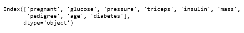

將輸出變量映射到0和1 (Mapping output variable into 0 and 1)

Before proceeding to model fitting, it is often essential to ensure that the data type is consistent with the library/package that you are going to use. In diabetes, data set the dependent variable (diabetes) consists of strings/characters i.e., neg/pos, which need to be converted into integers by mapping neg: 0 and pos: 1 using the .map( ) method.

在進行模型擬合之前，通常必須確保數據類型與要使用的庫/包一致。 在糖尿病中，數據集因變量(糖尿病)由字符串/字符(即neg / pos )組成，需要使用.map()方法通過映射neg：0和pos：1將其轉換為整數。

diabetes["diabetes"] = diabetes["diabetes"].map({"neg":0, "pos":1})diabetes["diabetes"].value_counts()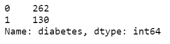

Now you can see that the dependent variable “diabetes” is converted from object to an integer 64 type.

現在您可以看到因變量“ diabetes ”從對象轉換為整數64類型。

The next step is to gaining knowledge about basic data summary statistics using .describe( ) method, which computes count, mean, standard deviation, minimum, maximum and percentile (25th, 50th and 75th) values. This helps you to detect any anomaly in your dataset. Such as variables with high variance or extremely skewed data.

下一步是使用.describe()方法獲取有關基本數據摘要統計信息的知識，該方法計算計數，均值，標準差，最小值，最大值和百分位數(第25、50和75位)。 這可以幫助您檢測數據集中的任何異常。 例如具有高方差的變量或數據嚴重偏斜。

訓練射頻模型 (Training RF Model)

The next step is splitting the diabetes data set into train and test split using train_test_split of sklearn.model_selection module and fitting a random forest model using the sklearn package/library.

下一步是分裂糖尿病數據集到列車和使用sklearn.model_selection模塊的train_test_split以及使用該sklearn包/庫擬合隨機森林模型試驗分裂。

訓練和測試拆分 (Train and Test Split)

The whole data set generally split into 80% train and 20% test data set (general rule of thumb). The 80% train data is being used for model training, while the rest 20% could be used for model generalized and local model interpretation.

整個數據集通常分為80％的訓練數據集和20％的測試數據集(一般經驗法則)。 80％的訓練數據用于模型訓練，而其余20％的數據可用于模型概括和局部模型解釋。

Y = diabetes['diabetes']
X = diabetes[['pregnant', 'glucose', 'pressure', 'triceps', 'insulin', 'mass',
       'pedigree', 'age']]X_featurenames = X.columns# Split the data into train and test data:
X_train, X_test, Y_train, Y_test = train_test_split(X, Y, test_size = 0.2)

In order to fit a Random Forest model, first, you need to install sklearn package/library and then you need to import RandomForestClassifier from sklearn.ensemble. Here, have fitted around 10000 trees with a max depth of 20.

為了適應隨機森林模型，首先，您需要安裝sklearn包/庫，那么你需要從sklearn.ensemble進口RandomForestClassifier。 這里， 已安裝約10000棵樹，最大深度為20。

# Build the model with the random forest regression algorithm:
model = RandomForestClassifier(max_depth = 20, random_state = 0, n_estimators = 10000)
model.fit(X_train, Y_train)

分類報告 (Classification Report)

Let’s predict the test data class labels using predict( ) and generate a classification report. The classification report revealed that the micro average of F1 score (used for unbalanced data) is about 0.71, which indicates that the trained model has a classification strength of 71%.

讓我們使用predict()預測測試數據類標簽并生成分類報告。 分類報告顯示，F1評分的微觀平均值(用于不平衡數據)約為0.71，這表明訓練后的模型的分類強度為71％。

y_pred = model.predict(X_test)print(classification_report(Y_test, y_pred, target_names=["Diabetes -ve", "Diabetes +ve"]))

特征重要性圖 (Feature Importance Plot)

The advantage of tree-based algorithms is that it provides global variable importance, which means you can rank them based on their contribution to the model. Here, you can observe that the glucose variable has the highest influence in the model, followed by Insulin. The problem with global importance is that it gives an average overview of variable contributing to the model.

基于樹的算法的優勢在于它提供了全局變量重要性，這意味著您可以根據它們對模型的貢獻對其進行排名。 在這里，您可以觀察到葡萄糖變量在模型中影響最大，其次是胰島素 。 具有全球重要性的問題是，它給出了有助于模型的變量的平均概圖。

feat_importances = pd.Series(model.feature_importances_, index = X_featurenames)feat_importances.nlargest(5).plot(kind = 'barh')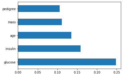

From the BlackBox model, it is nearly impossible to get a feeling for its inner functioning. This brings us to a question of trust: do you trust that a certain prediction from the model is correct? Or do you even trust that the model is making sound predictions?

從BlackBox模型中，幾乎不可能對它的內部功能有所了解。 這給我們帶來了一個信任問題：您是否相信模型中的某個預測是正確的？ 還是您甚至相信模型可以做出合理的預測？

創建一個模型解釋器 (Creating a model explainer)

LIME is short for Local Interpretable Model-Agnostic Explanations. Local refers to local fidelity — i.e., we want the explanation to really reflect the behaviour of the classifier “around” the instance being predicted. This explanation is useless unless it is interpretable — that is, unless a human can make sense of it. Lime is able to explain any model without needing to ‘peak’ into it, so it is model-agnostic.

LIME是本地可解釋模型不可知的解釋的縮寫。 本地是指本地保真度-即，我們希望解釋能真正反映分類器在“預測”實例周圍的行為。 除非可以解釋 ，否則這種解釋是無用的，也就是說，除非人類可以理解。 Lime能夠解釋任何模型而無需“說話”，所以它與模型無關 。

Behind the workings of LIME lies the assumption that every complex model is linear on a local scale and asserting that it is possible to fit a simple model around a single observation that will mimic how the global model behaves at that locality (Pedersen and Benesty, 2016)

LIME的工作原理是，假設每個復雜模型在局部范圍內都是線性的，并斷言有可能在單個觀測值附近擬合一個簡單模型，以模擬全局模型在該位置的行為(Pedersen和Benesty，2016年) )

LIME explainer fitting steps

LIME解釋器安裝步驟

• import the lime library
  導入石灰庫
• import lime.lime_tabular
  導入lime.lime_tabular

• Fit an explainer using LimeTabularExplainer( ) function

  使用LimeTabularExplainer()函數擬合解釋器

• Supply the x_train values, feature names and class names as ‘Diabetes -ve’, ‘Diabetes +ve’

  提供x_train值， 特征名稱和類名稱，例如' Diabetes -ve '，' Diabetes + ve '

• Here we used the lasso_path for feature selection

  這里我們使用lasso_path進行特征選擇

• binned continuous variable into discrete values (discretize_continuous = True) based on “quartile”

  根據“ 四分位數 ”將連續變量分為離散值( discretize_continuous = True )

• Select mode as classification

  選擇模式作為分類

import limeimport lime.lime_tabularexplainer = lime.lime_tabular.LimeTabularExplainer(X_train.values, feature_names = X_featurenames, class_names = ['Diabetes -ve', 'Diabetes +ve'], feature_selection = "lasso_path", discretize_continuous = True, discretizer = "quartile", verbose = True, mode = 'classification')

For local level explanation let’s pick an observation from test data who is diabetes +ve. Let’s select the 3rd observation (index 254). Here are the first 5 observations from X_test dataset including 3rd observation (index number 254)

對于局部級別的解釋，讓我們從測試數據中選擇一個觀察者，即糖尿病+ ve。 讓我們選擇第三個觀察值(索引254)。 這是X_test數據集中的前5個觀察值，包括第3個觀察值(索引號254)

X_test.iloc[0:5]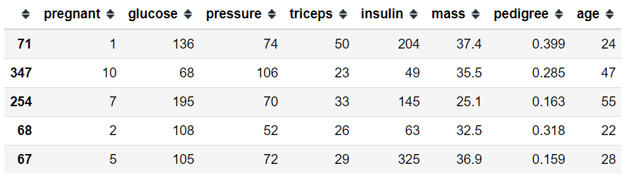

Let’s observe the output variable. You can observe the 3rd observation (index 254) has a value of 1 which indicates it is diabetes +ve.

讓我們觀察一下輸出變量。 您可以觀察到第三個觀察值(索引254)的值為1，表示糖尿病+ ve。

Y_test.iloc[0:5]

Let’s see whether LIME able to interpret which variables contribute to +ve diabetes and what is the impact magnitude and direction for observation 3 (index number 254)

讓我們看看LIME是否能夠解釋哪些變量導致+ ve糖尿病，以及觀察的影響幅度和方向是什么(索引號254)3

解釋第一個觀察 (Explain the first observation)

For model explanation, one needs to supply the observation and the model predicted probabilities.

為了進行模型解釋，需要提供觀察值和模型預測的概率。

The output shows the local level LIME model intercept is 0.245 and LIME model prediction is 0.613 (Prediction_local). The original random forest model prediction 0.589. Now, we can plot the explaining variables to show their contribution. In the plot, the right side green bar shows support for +ve diabetes while left side red bars contradicts the support. The variable glucose > 142 shows the highest support for +ve diabetes for the selected observation. In other words for observation 3 in the test dataset having glucose> 142 primarily contributed to +ve diabetes.

輸出顯示本地級別的LIME模型截距為0.245，而LIME模型的預測值為0.613(Prediction_local)。 原始隨機森林模型預測值為0.589。 現在，我們可以繪制解釋變量以顯示它們的作用。 在該圖中，右側的綠色條表示對+ ve糖尿病的支持，而左側的紅色條與支持相反。 對于選定的觀察，可變葡萄糖> 142顯示對+ ve糖尿病的最高支持。 換句話說，對于葡萄糖> 142的測試數據集中的觀察3，其主要導致+ ve糖尿病。

exp = explainer.explain_instance(X_test.iloc[2], model.predict_proba)exp.as_pyplot_figure()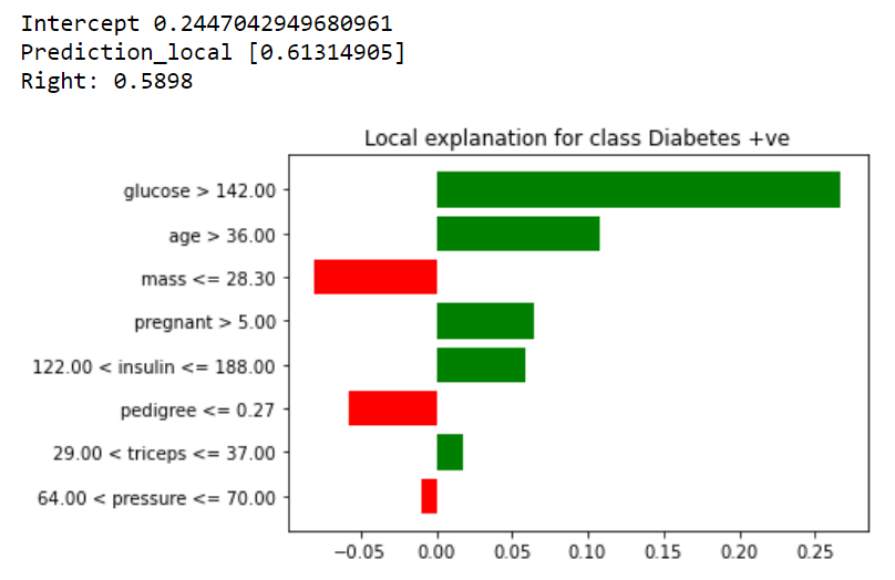

Similarly, you can plot a detailed explanation using the show_in_notebook( ) function.

同樣，您可以使用show_in_notebook()函數繪制詳細說明。

exp = explainer.explain_instance(X_test.iloc[2], model.predict_proba)exp.show_in_notebook(show_table = True, show_all = False)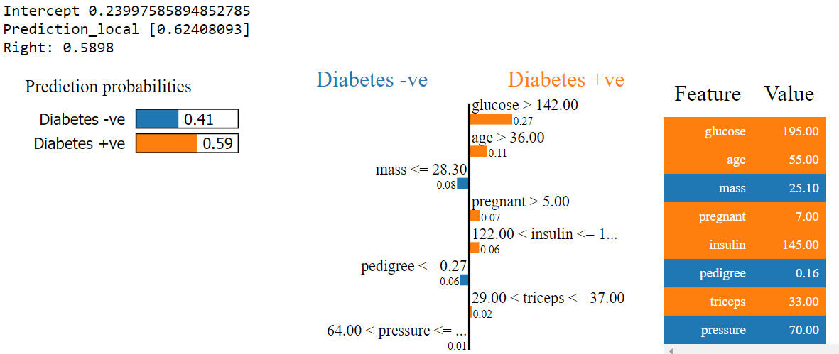

In summary, black-box models nowadays not a black box anymore. There are plenty of algorithms that have been proposed by researchers. Some of them are LIME, Sharp values etc. The above explanation mechanism could be used for all major classification and regression algorithms, even for the deep neural networks.

總而言之，黑匣子模型如今已不再是黑匣子了。 研究人員已經提出了許多算法。 其中一些是LIME，Sharp值等。以上解釋機制可用于所有主要的分類和回歸算法，甚至適用于深度神經網絡。

If you learned something new and liked this article, follow on Twitter, LinkedIn, YouTube or Github.

如果您學到了新知識并喜歡本文，請在Twitter ， LinkedIn ， YouTube 或 Github上關注 。

Note

注意

This article was first published on onezero.blog, a data science, machine learning and research related blogging platform maintained by me.

本文首次發表于onezero.blog ，數據科學，機器學習和研究相關的博客平臺維護由我。

More Interesting Readings — I hope you’ve found this article useful! Below are some interesting readings hope you like them too —

更多有趣的讀物 - 希望您對本文有所幫助！ 以下是一些有趣的讀物，希望您也喜歡 -