This post aims to explore a step-by-step approach to create a K-Nearest Neighbors Algorithm without the help of any third-party library. In practice, this Algorithm should be useful enough for us to classify our data whenever we have already made classifications (in this case, color), which will serve as a starting point to find neighbors.

這篇文章旨在探索逐步方法，以在無需任何第三方庫的幫助下創建K最近鄰居算法 。 在實踐中，只要我們已經進行了分類(在這種情況下為顏色)，該算法就足以對我們進行數據分類，這將成為尋找鄰居的起點。

For this post, we will use a specific dataset which can be downloaded here. It contains 539 two dimensional data points, each with a specific color classification. Our goal will be to separate them into two groups (train and test) and try to guess our test sample colors based on our algorithm recommendation.

對于這篇文章，我們將使用一個特定的數據集，可以在此處下載 。 它包含539個二維數據點，每個數據點都有特定的顏色分類。 我們的目標是將它們分為兩組(訓練和測試)，并根據算法建議嘗試猜測測試樣本的顏色。

訓練和測試樣品生成 (Train and test sample generation)

We will create two different sample sets:

我們將創建兩個不同的樣本集：

• Training Set: This will contain 75% of our working data, selected randomly. This set will be used to generate our model.

  訓練集：這將包含我們75％的工作數據，是隨機選擇的。 該集合將用于生成我們的模型。

• Test Set: Remaining 25% of our working data will be used to test the out-of-sample accuracy of our model. Once our predictions of this 25% are made, we will check the “percentage of correct classifications” by comparing predictions versus real values.

  測試集：我們剩余的25％的工作數據將用于測試模型的樣本外準確性。 一旦做出25％的預測，我們將通過比較預測值與實際值來檢查“ 正確分類的百分比 ”。

# Load Data
library(readr)
RGB <- as.data.frame(read_csv("RGB.csv"))
RGB$x <- as.numeric(RGB$x)
RGB$y <- as.numeric(RGB$y)
print("Working data ready")# Training Dataset
smp_siz = floor(0.75*nrow(RGB))
train_ind = sample(seq_len(nrow(RGB)),size = smp_siz)
train =RGB[train_ind,]# Testting Dataset
test=RGB[-train_ind,]
OriginalTest <- test
paste("Training and test sets done")

訓練數據 (Training Data)

We can observe that our train data is classified into 3 clusters based on colors.

我們可以觀察到，我們的火車數據基于顏色分為3類。

# We plot test colored datapoints
library(ggplot2)
colsdot <- c("Blue" = "blue", "Red" = "darkred", "Green" = "darkgreen")
ggplot() + 
  geom_tile(data=train,mapping=aes(x, y), alpha=0) +
  ##Ad tiles according to probabilities
  ##add points
  geom_point(data=train,mapping=aes(x,y, colour=Class),size=3 ) + 
  scale_color_manual(values=colsdot) +
  #add the labels to the plots
  xlab('X') + ylab('Y') + ggtitle('Train Data')+
  #remove grey border from the tile
  scale_x_continuous(expand=c(0,.05))+scale_y_continuous(expand=c(0,.05))

測試數據 (Test Data)

Even though we know the original color classification of our test data, we will try to create a model that can guess its color based solely on an educated guess. For this, we will remove their original colors and save them only for testing purposes; once our model makes its prediction, we will be able to calculate our Model Accuracy by comparing the original versus our prediction.

即使我們知道測試數據的原始顏色分類，我們也將嘗試創建一個僅可以根據有根據的猜測來猜測其顏色的模型。 為此，我們將刪除其原始顏色，并僅將其保存以用于測試； 一旦我們的模型做出了預測，我們就可以通過比較原始預測和我們的預測來計算模型精度 。

# We plot test colored datapoints
colsdot <- c("Blue" = "blue", "Red" = "darkred", "Green" = "darkgreen")
ggplot() + 
  geom_tile(data=test,mapping=aes(x, y), alpha=0) +
  ##Ad tiles according to probabilities
  ##add points
  geom_point(data=test,mapping=aes(x,y),size=3 ) + 
  scale_color_manual(values=colsdot) +
  #add the labels to the plots
  xlab('X') + ylab('Y') + ggtitle('Test Data')+
  #remove grey border from the tile
  scale_x_continuous(expand=c(0,.05))+scale_y_continuous(expand=c(0,.05))

K最近鄰居算法 (K-Nearest Neighbors Algorithm)

Below is a step-by-step example of an implementation of this algorithm. What we want to achieve is for each selected gray point above (our test values), where we allegedly do not know their actual color, find the nearest neighbor or nearest colored data point from our train values and assign the same color as this one.

下面是該算法實現的分步示例。 我們想要實現的是針對上面每個選定的灰點(我們的測試值)，據稱我們不知道它們的實際顏色，從我們的火車值中找到最近的鄰居或最接近的彩色數據點，并為其分配相同的顏色。

In particular, we need to:

特別是，我們需要：

• Normalize data: even though in this case is not needed, since all values are in the same scale (decimals between 0 and 1), it is recommended to normalize in order to have a “standard distance metric”.

  歸一化數據：即使在這種情況下不需要，由于所有值都在相同的標度(0到1之間的小數)，建議進行歸一化以具有“標準距離度量”。

• Define how we measure distance: We can define the distance between two points in this two-dimensional data set as the Euclidean distance between them. We will calculate L1 (sum of absolute differences) and L2 (sum of squared differences) distances, though final results will be calculated using L2 since its more unforgiving than L1.

  定義測量距離的方式：我們可以將此二維數據集中的兩個點之間的距離定義為它們之間的歐式距離。 我們將計算L1(絕對差之和)和L2(平方差之和)的距離，盡管最終結果將使用L2來計算，因為它比L1更加不容忍。

• Calculate Distances: we need to calculate the distance between each tested data point and every value within our train dataset. Normalization is critical here since, in the case of body structure, a distance in weight (1 KG) and height (1 M) is not comparable. We can anticipate a higher deviation in KG than it is on the Meters, leading to incorrect overall distances.

  計算距離：我們需要計算每個測試數據點與火車數據集中每個值之間的距離。 歸一化在這里至關重要，因為在身體結構的情況下，重量(1 KG)和高度(1 M)的距離不可比。 我們可以預期到KG的偏差要比儀表多，從而導致總距離不正確。

• Sort Distances: Once we calculate the distance between every test and training points, we need to sort them in descending order.

  距離排序：一旦我們計算出每個測試點與訓練點之間的距離，就需要對它們進行降序排序。

• Selecting top K nearest neighbors: We will select the top K nearest train data points to inspect which category (colors) they belong to in order also to assign this category to our tested point. Since we might use multiple neighbors, we might end up with multiple categories, in which case, we should calculate a probability.

  選擇最接近的K個最近的鄰居：我們將選擇最接近的K個火車數據點來檢查它們屬于哪個類別(顏色)，以便將該類別分配給我們的測試點。 由于我們可能使用多個鄰居，因此我們可能會得到多個類別，在這種情況下，我們應該計算一個概率。

# We define a function for prediction
KnnL2Prediction <- function(x,y,K) {
    
  # Train data
  Train <- train
  # This matrix will contain all X,Y values that we want test.
  Test <- data.frame(X=x,Y=y)
    
  # Data normalization
  Test$X <- (Test$X - min(Train$x))/(min(Train$x) - max(Train$x))
  Test$Y <- (Test$Y - min(Train$y))/(min(Train$y) - max(Train$y))
  Train$x <- (Train$x - min(Train$x))/(min(Train$x) - max(Train$x))
  Train$y <- (Train$y - min(Train$y))/(min(Train$y) - max(Train$y))  # We will calculate L1 and L2 distances between Test and Train values.
  VarNum <- ncol(Train)-1
  L1 <- 0
  L2 <- 0
  for (i in 1:VarNum) {
    L1 <- L1 + (Train[,i] - Test[,i])
    L2 <- L2 + (Train[,i] - Test[,i])^2
  }
    
  # We will use L2 Distance
  L2 <- sqrt(L2)
  
  # We add labels to distances and sort
  Result <- data.frame(Label=Train$Class,L1=L1,L2=L2)
  
  # We sort data based on score
  ResultL1 <-Result[order(Result$L1),]
  ResultL2 <-Result[order(Result$L2),]
  
  # Return Table of Possible classifications
  a <- prop.table(table(head(ResultL2$Label,K)))
  b <- as.data.frame(a)
  return(as.character(b$Var1[b$Freq == max(b$Freq)]))
}

使用交叉驗證找到正確的K參數 (Finding the correct K parameter using Cross-Validation)

For this, we will use a method called “cross-validation”. What this means is that we will make predictions within the training data itself and iterate this on many different values of K for many different folds or permutations of the data. Once we are done, we will average our results and obtain the best K for our “K-Nearest” Neighbors algorithm.

為此，我們將使用一種稱為“交叉驗證”的方法。 這意味著我們將在訓練數據本身中進行預測，并針對數據的許多不同折疊或排列對許多不同的K值進行迭代。 完成之后，我們將平均結果并為“ K最近”鄰居算法獲得最佳K。

# We will use 5 folds
FoldSize = floor(0.2*nrow(train)) # Fold1
piece1 = sample(seq_len(nrow(train)),size = FoldSize ) 
Fold1 = train[piece1,]
rest = train[-piece1,] # Fold2
piece2 = sample(seq_len(nrow(rest)),size = FoldSize)
Fold2 = rest[piece2,]
rest = rest[-piece2,] # Fold3
piece3 = sample(seq_len(nrow(rest)),size = FoldSize)
Fold3 = rest[piece3,]
rest = rest[-piece3,] # Fold4
piece4 = sample(seq_len(nrow(rest)),size = FoldSize)
Fold4 = rest[piece4,]
rest = rest[-piece4,] # Fold5
Fold5 <- rest# We make folds
Split1_Test <- rbind(Fold1,Fold2,Fold3,Fold4)
Split1_Train <- Fold5Split2_Test <- rbind(Fold1,Fold2,Fold3,Fold5)
Split2_Train <- Fold4Split3_Test <- rbind(Fold1,Fold2,Fold4,Fold5)
Split3_Train <- Fold3Split4_Test <- rbind(Fold1,Fold3,Fold4,Fold5)
Split4_Train <- Fold2Split5_Test <- rbind(Fold2,Fold3,Fold4,Fold5)
Split5_Train <- Fold1# We select best K
OptimumK <- data.frame(K=NA,Accuracy=NA,Fold=NA)
results <- trainfor (i in 1:5) {
  if(i == 1) {
    train <- Split1_Train
    test <- Split1_Test
  } else if(i == 2)  {
    train <- Split2_Train
    test <- Split2_Test
  } else if(i == 3)  {
    train <- Split3_Train
    test <- Split3_Test
  } else if(i == 4)  {
    train <- Split4_Train
    test <- Split4_Test
  } else if(i == 5)  {
    train <- Split5_Train
    test <- Split5_Test
  }
    for(j in 1:20) {
      results$Prediction <- mapply(KnnL2Prediction, results$x, results$y,j)
      # We calculate accuracy
      results$Match <- ifelse(results$Class == results$Prediction, 1, 0)
      Accuracy <- round(sum(results$Match)/nrow(results),4)
      OptimumK <- rbind(OptimumK,data.frame(K=j,Accuracy=Accuracy,Fold=paste("Fold",i)))
    
    }
}OptimumK <- OptimumK [-1,]
MeanK <- aggregate(Accuracy ~ K, OptimumK, mean)
ggplot() + 
  geom_point(data=OptimumK,mapping=aes(K,Accuracy, colour=Fold),size=3 ) +
  geom_line(aes(K, Accuracy, colour="Moving Average"), linetype="twodash", MeanK) +
  scale_x_continuous(breaks=seq(1, max(OptimumK$K), 1))

As seen in the plot above, we can observe that our algorithm’s prediction accuracy is in the range of 88%-95% for all folds and decreasing from K=3 onwards. We can observe the highest consistent accuracy results on K=1 (3 is also a good alternative).

如上圖所示，我們可以觀察到我們算法的所有折疊的預測準確度都在88％-95％的范圍內，并且從K = 3開始下降。 我們可以在K = 1上觀察到最高的一致精度結果(3也是一個很好的選擇)。

根據最近的1個鄰居進行預測。 (Predicting based on Top 1 Nearest Neighbors.)

模型精度 (Model Accuracy)

# Predictions over our Test sample
test <- OriginalTest
K <- 1
test$Prediction <- mapply(KnnL2Prediction, test$x, test$y,K)
head(test,10)# We calculate accuracy
test$Match <- ifelse(test$Class == test$Prediction, 1, 0)
Accuracy <- round(sum(test$Match)/nrow(test),4)
print(paste("Accuracy of ",Accuracy*100,"%",sep=""))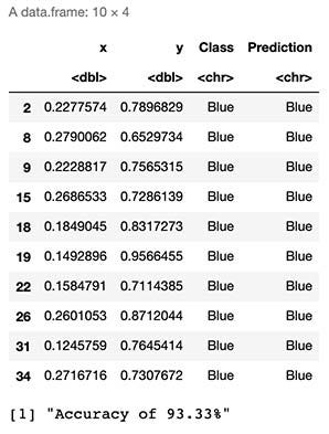

As seen by the results above, we can expect to “guess the correct class or color” 93% of the time.

從上面的結果可以看出，我們可以期望在93％的時間內“猜測正確的類別或顏色”。

原始色彩 (Original Colors)

Below we can observe the original colors or classes of our test sample.

下面我們可以觀察測試樣??品的原始顏色或類別。

ggplot() + 
  geom_tile(data=test,mapping=aes(x, y), alpha=0) +
  geom_point(data=test,mapping=aes(x,y,colour=Class),size=3 ) + 
  scale_color_manual(values=colsdot) +
  xlab('X') + ylab('Y') + ggtitle('Test Data')+
  scale_x_continuous(expand=c(0,.05))+scale_y_continuous(expand=c(0,.05))

預測的顏色 (Predicted Colors)

Using our algorithm, we obtain the following colors for our initially colorless sample dataset.

使用我們的算法，我們為最初的無色樣本數據集獲得了以下顏色。

ggplot() + 
  geom_tile(data=test,mapping=aes(x, y), alpha=0) +
  geom_point(data=test,mapping=aes(x,y,colour=Prediction),size=3 ) + 
  scale_color_manual(values=colsdot) +
  xlab('X') + ylab('Y') + ggtitle('Test Data')+
  scale_x_continuous(expand=c(0,.05))+scale_y_continuous(expand=c(0,.05))

As seen in the plot above, it seems even though our algorithm correctly classified most of the data points, it failed with some of them (marked in red).

如上圖所示，即使我們的算法正確地對大多數數據點進行了分類，但其中的某些數據點還是失敗了(用紅色標記)。

決策極限 (Decision Limits)

Finally, we can visualize our “decision limits” over our original Test Dataset. This provides an excellent visual approximation of how well our model is classifying our data and the limits of its classification space.

最后，我們可以可視化我們原始測試數據集上的“決策限制”。 這為模型對數據的分類及其分類空間的局限性提供了極好的視覺近似。

In simple words, we will simulate 160.000 data points (400x400 matrix) within the range of our original dataset, which, when later plotted, will fill most of the empty spaces with colors. This will help us express in detail how our model would classify this 2D space within it’s learned color classes. The more points we generate, the better our “resolution” will be, much like pixels on a TV.

簡而言之，我們將在原始數據集范圍內模擬160.000個數據點(400x400矩陣)，當稍后繪制時，這些數據點將用顏色填充大部分空白空間。 這將幫助我們詳細表達我們的模型如何在其學習的顏色類別中對該2D空間進行分類。 我們生成的點越多，我們的“分辨率”就越好，就像電視上的像素一樣。

# We calculate background colors
x_coord = seq(min(train[,1]) - 0.02,max(train[,1]) + 0.02,length.out = 40)
y_coord = seq(min(train[,2]) - 0.02,max(train[,2]) + 0.02, length.out = 40)
coord = expand.grid(x = x_coord, y = y_coord)
coord[['prob']] = mapply(KnnL2Prediction, coord$x, coord$y,K)# We calculate predictions and plot decition area
colsdot <- c("Blue" = "blue", "Red" = "darkred", "Green" = "darkgreen")
colsfill <- c("Blue" = "#aaaaff", "Red" = "#ffaaaa", "Green" = "#aaffaa")
ggplot() + 
  geom_tile(data=coord,mapping=aes(x, y, fill=prob), alpha=0.8) +
  geom_point(data=test,mapping=aes(x,y, colour=Class),size=3 ) + 
  scale_color_manual(values=colsdot) +
  scale_fill_manual(values=colsfill) +
  xlab('X') + ylab('Y') + ggtitle('Decision Limits')+
  scale_x_continuous(expand=c(0,0))+scale_y_continuous(expand=c(0,0))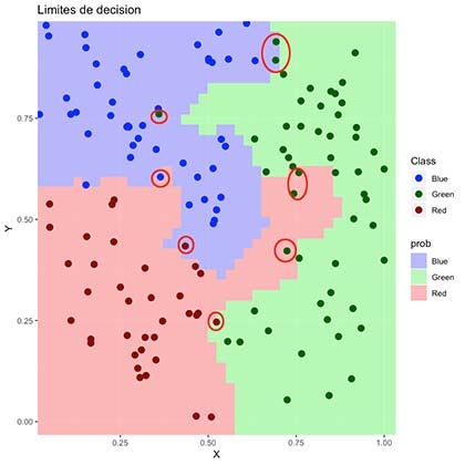

As seen above, the colored region represents which areas our algorithm would define as a “colored data point”. It is visible why it failed to classify some of them correctly.

如上所示，彩色區域表示我們的算法將哪些區域定義為“彩色數據點”。 可見為什么無法正確分類其中一些。

最后的想法 (Final Thoughts)

K-Nearest Neighbors is a straightforward algorithm that seems to provide excellent results. Even though we can classify items by eye here, this model also works in cases of higher dimensions where we cannot merely observe them by the naked eye. For this to work, we need to have a training dataset with existing classifications, which we will later use to classify data around it, meaning it is a supervised machine learning algorithm.

K最近鄰居是一種簡單的算法，似乎可以提供出色的結果。 即使我們可以在這里按肉眼對項目進行分類，該模型也可以在無法僅用肉眼觀察它們的較高維度的情況下使用。 為此，我們需要有一個帶有現有分類的訓練數據集，稍后我們將使用它來對周圍的數據進行分類 ，這意味著它是一種監督式機器學習算法 。

Sadly, this method presents difficulties in scenarios such as in the presence of intricate patterns that cannot be represented by simple straight distance, like in the cases of radial or nested clusters. It also has the problem of performance since, for every classification of a new data point, we need to compare it to every single point in our training dataset, which is resource and time intensive since it requires replication and iteration of the complete set.

可悲的是，這種方法在諸如無法以簡單直線距離表示的復雜圖案的情況下(例如在徑向或嵌套簇的情況下)會遇到困難。 它也存在性能問題，因為對于新數據點的每個分類，我們都需要將其與訓練數據集中的每個點進行比較，這是資源和時間密集的，因為它需要復制和迭代整個集合。