Polynomial regression in an improved version of linear regression. If you know linear regression, it will be simple for you. If not, I will explain the formulas here in this article. There are other advanced and more efficient machine learning algorithms are out there. But it is a good idea to learn linear based regression techniques. Because they are simple, fast, and works with very well known formulas. Though it may not work with a complex set of data.

線性回歸的改進版本中的多項式回歸。 如果您知道線性回歸，那么對您來說很簡單。 如果沒有，我將在本文中解釋這些公式。 還有其他先進且更有效的機器學習算法。 但是，學習基于線性的回歸技術是一個好主意。 因為它們簡單，快速并且可以使用眾所周知的公式。 盡管它可能不適用于復雜的數據集。

多項式回歸公式 (Polynomial Regression Formula)

Linear regression can perform well only if there is a linear correlation between the input variables and the output variable. As I mentioned before polynomial regression is built on linear regression. If you need a refresher on linear regression, here is the link to linear regression:

僅當輸入變量和輸出變量之間存在線性相關性時，線性回歸才能很好地執行。 如前所述，多項式回歸建立在線性回歸的基礎上。 如果您需要線性回歸的基礎知識，請訪問以下線性回歸鏈接：

Polynomial regression can find the relationship between input features and the output variable in a better way even if the relationship is not linear. It uses the same formula as the linear regression:

多項式回歸可以更好地找到輸入要素與輸出變量之間的關系，即使該關系不是線性的。 它使用與線性回歸相同的公式：

Y = BX + C

Y = BX + C

I am sure, we all learned this formula in school. For linear regression, we use symbols like this:

我敢肯定，我們都在學校學過這個公式。 對于線性回歸，我們使用如下符號：

Here, we get X and Y from the dataset. X is the input feature and Y is the output variable. Theta values are initialized randomly.

在這里，我們從數據集中獲得X和Y。 X是輸入要素，Y是輸出變量。 Theta值是隨機初始化的。

For polynomial regression, the formula becomes like this:

對于多項式回歸，公式如下所示：

We are adding more terms here. We are using the same input features and taking different exponentials to make more features. That way, our algorithm will be able to learn about the data better.

我們在這里添加更多術語。 我們使用相同的輸入功能，并采用不同的指數以制作更多功能。 這樣，我們的算法將能夠更好地了解數據。

The powers do not have to be 2, 3, or 4. They could be 1/2, 1/3, or 1/4 as well. Then the formula will look like this:

冪不必為2、3或4。它們也可以為1 / 2、1 / 3或1/4。 然后，公式將如下所示：

成本函數和梯度下降 (Cost Function And Gradient Descent)

Cost function gives an idea of how far the predicted hypothesis is from the values. The formula is:

成本函數給出了預測假設與值之間的距離的概念。 公式為：

This equation may look complicated. It is doing a simple calculation. First, deducting the hypothesis from the original output variable. Taking a square to eliminate the negative values. Then dividing that value by 2 times the number of training examples.

這個方程可能看起來很復雜。 它正在做一個簡單的計算。 首先，從原始輸出變量中減去假設。 取平方消除負值。 然后將該值除以訓練示例數的2倍。

What is gradient descent? It helps in fine-tuning our randomly initialized theta values. I am not going to the differential calculus here. If you take the partial differential of the cost function on each theta, we can derive these formulas:

什么是梯度下降？ 它有助于微調我們隨機初始化的theta值。 我不打算在這里進行微積分。 如果對每個θ取成本函數的偏微分，則可以得出以下公式：

Here, alpha is the learning rate. You choose the value of alpha.

在這里，alpha是學習率。 您選擇alpha的值。

多項式回歸的Python實現 (Python Implementation of Polynomial Regression)

Here is the step by step implementation of Polynomial regression.

這是多項式回歸的逐步實現。

1. We will use a simple dummy dataset for this example that gives the data of salaries for positions. Import the dataset:
   在此示例中，我們將使用一個簡單的虛擬數據集，該數據集提供職位的薪水數據。 導入數據集：

import pandas as pd
import numpy as np
df = pd.read_csv('position_salaries.csv')
df.head()

2. Add the bias column for theta 0. This bias column will only contain 1. Because if you multiply 1 with a number it does not change.

2.添加theta 0的偏差列。該偏差列將僅包含1。因為如果將1乘以數字，它不會改變。

df = pd.concat([pd.Series(1, index=df.index, name='00'), df], axis=1)
df.head()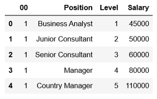

3. Delete the ‘Position’ column. Because the ‘Position’ column contains strings and algorithms do not understand strings. We have the ‘Level’ column to represent the positions.

3.刪除“位置”列。 由于“位置”列包含字符串，并且算法無法理解字符串。 我們有“級別”列來代表職位。

df = df.drop(columns='Position')

4. Define our input variable X and the output variable y. In this example, ‘Level’ is the input feature and ‘Salary’ is the output variable. We want to predict the salary for levels.

4.定義我們的輸入變量X和輸出變量y。 在此示例中，“級別”是輸入要素，而“薪水”是輸出變量。 我們要預測各個級別的薪水。

y = df['Salary']
X = df.drop(columns = 'Salary')
X.head()

5. Take the exponentials of the ‘Level’ column to make ‘Level1’ and ‘Level2’ columns.

5.以“級別”列的指數表示“級別1”和“級別2”列。

X['Level1'] = X['Level']**2
X['Level2'] = X['Level']**3
X.head()

6. Now, normalize the data. Divide each column by the maximum value of that column. That way, we will get the values of each column ranging from 0 to 1. The algorithm should work even without normalization. But it helps to converge faster. Also, calculate the value of m which is the length of the dataset.

6.現在，標準化數據。 將每一列除以該列的最大值。 這樣，我們將獲得每列的值，范圍從0到1。即使沒有規范化，該算法也應該起作用。 但這有助于收斂更快。 同樣，計算m的值，它是數據集的長度。

m = len(X)
X = X/X.max()

7. Define the hypothesis function. That will use the X and theta to predict the ‘y’.

7.定義假設函數。 這將使用X和theta來預測“ y”。

def hypothesis(X, theta):
    y1 = theta*X
    return np.sum(y1, axis=1)

8. Define the cost function, with our formula for cost-function above:

8.使用上面的成本函數公式定義成本函數：

def cost(X, y, theta):
    y1 = hypothesis(X, theta)
    return sum(np.sqrt((y1-y)**2))/(2*m)

9. Write the function for gradient descent. We will keep updating the theta values until we find our optimum cost. For each iteration, we will calculate the cost for future analysis.

9.編寫梯度下降函數。 我們將不斷更新theta值，直到找到最佳成本。 對于每次迭代，我們將計算成本以供將來分析。

def gradientDescent(X, y, theta, alpha, epoch):
    J=[]
    k=0
    while k < epoch:
        y1 = hypothesis(X, theta)
        for c in range(0, len(X.columns)):
            theta[c] = theta[c] - alpha*sum((y1-y)* X.iloc[:, c])/m
        j = cost(X, y, theta)
        J.append(j)
        k += 1
    return J, theta

10. All the functions are defined. Now, initialize the theta. I am initializing an array of zero. You can take any other random values. I am choosing alpha as 0.05 and I will iterate the theta values for 700 epochs.

10.定義了所有功能。 現在，初始化theta。 我正在初始化零數組。 您可以采用任何其他隨機值。 我選擇alpha為0.05，我將迭代700個紀元的theta值。

theta = np.array([0.0]*len(X.columns))
J, theta = gradientDescent(X, y, theta, 0.05, 700)

11. We got our final theta values and the cost in each iteration as well. Let’s find the salary prediction using our final theta.

11.我們還獲得了最終的theta值以及每次迭代的成本。 讓我們使用最終的theta查找薪水預測。

y_hat = hypothesis(X, theta)

12. Now plot the original salary and our predicted salary against the levels.

12.現在根據水平繪制原始薪水和我們的預測薪水。

%matplotlib inline
import matplotlib.pyplot as plt
plt.figure()
plt.scatter(x=X['Level'],y= y)           
plt.scatter(x=X['Level'], y=y_hat)
plt.show()

Our prediction does not exactly follow the trend of salary but it is close. Linear regression can only return a straight line. But in polynomial regression, we can get a curved line like that. If the line would not be a nice curve, polynomial regression can learn some more complex trends as well.

我們的預測并不完全符合薪資趨勢，但接近。 線性回歸只能返回一條直線。 但是在多項式回歸中，我們可以得到這樣的曲線。 如果該線不是一條好曲線，則多項式回歸也可以學習一些更復雜的趨勢。

13. Let’s plot the cost we calculated in each epoch in our gradient descent function.

13.讓我們繪制我們在梯度下降函數中每個時期計算的成本。

plt.figure()
plt.scatter(x=list(range(0, 700)), y=J)
plt.show()

The cost fell drastically in the beginning and then the fall was slow. In a good machine learning algorithm, cost should keep going down until the convergence. Please feel free to try it with a different number of epochs and different learning rates (alpha).

成本從一開始就急劇下降，然后下降緩慢。 在一個好的機器學習算法中，成本應該一直下降直到收斂。 請隨意嘗試不同的時期和不同的學習率(alpha)。

Here is the dataset: salary_data

這是數據集： salary_data

Follow this link for the full working code: Polynomial Regression

請點擊以下鏈接獲取完整的工作代碼： 多項式回歸

推薦閱讀： (Recommended reading:)