What’s the future of the world’s coral reefs?

世界珊瑚礁的未來是什么？

In February of 2020, scientists at University of Hawaii Manoa released a study addressing this very question. The models they developed forecasted a 70–90% worldwide loss of coral by 2040. Even more alarming, they projected that “few to zero suitable coral habitats will remain” by the year 2100.

2020年2月，夏威夷大學馬諾阿分校的科學家發布了一項針對這一問題的研究 。 他們開發的模型預測，到2040年，全球珊瑚損失將達到70-90％。更令人震驚的是，他們預測，到2100年，“將幾乎沒有零個合適的珊瑚棲息地”。

So, the future of coral doesn’t look great.

因此，珊瑚的未來看起來并不美好。

Interested in seeing these numbers firsthand, today we will develop our own forecasts of hard corals in the Caribbean. After restructuring the data, we’ll fit an extremely famous time series model: ARIMA. ARIMA has been popularized due to its simplicity and specific ability to fit time series data. Once we have a working model, we’ll develop a forecast.

有興趣直接看到這些數字，今天我們將對加勒比地區的硬珊瑚進行預測。 重組數據后，我們將擬合一個非常著名的時間序列模型： ARIMA 。 由于ARIMA的簡單性和適應時間序列數據的特定能力，它已得到普及。 建立工作模型后，我們將進行預測。

Let’s jump right in.

讓我們跳進去。

為什么需要匯總？ (Why do you need to aggregate?)

We’ll start by taking a look at our raw data. In this case, we are going to be building a univariate model, so we’re only concerned with hard coral percent cover (i.e. the estimated percentage of hard coral on the sea floor).

我們將從查看原始數據開始。 在這種情況下，我們將建立一個單變量模型，因此我們只關心硬珊瑚百分比覆蓋率(即海底硬珊瑚的估計百分比)。

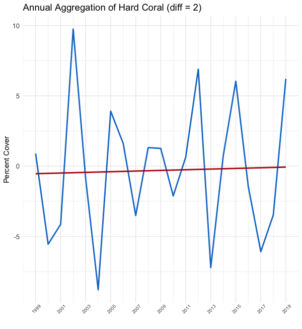
In the figure to the left, we have plotted the daily average of hard coral over time (blue). The y-axis shows the percent cover and the x-axis shows the date, ranging from 1997–2019. We also plotted a weighted linear regression line (red) to depict the overall trend.

在左圖中，我們繪制了一段時間內硬珊瑚的日平均值(藍色)。 y軸顯示覆蓋率百分比，x軸顯示日期，范圍為1997–2019。 我們還繪制了加權線性回歸線(紅色)以描繪總體趨勢。

Ok, seems straight-forward.

好吧，似乎很簡單。

But if we try to interpret these data, we see a blue mess with a negative trend line; there appears to be little systematic movement. Moreover, according to the regression line, hard coral only decreased by around 4% over the past 22 years. That’s pretty hard to believe. So, as creative and skilled data scientists, let’s try some manipulations and see if we can develop a clearer picture.

但是，如果我們嘗試解釋這些數據，則會看到藍色的混亂趨勢線為負； 似乎很少有系統的運動。 此外，根據回歸線，硬珊瑚在過去22年中僅下降了約4％。 很難相信。 因此，作為富有創造力和技能的數據科學家，讓我們嘗試一些操作，看看是否可以得出更清晰的圖景。

First, it’s important to know how the data are organized. Unlike most time series datasets, these data were sampled at different locations around the Caribbean with few subsequent draws at the same site. Moreover, they are not equally sampled over time. So, to account for the above points, let’s aggregate the data by time.

首先，了解數據的組織方式非常重要。 與大多數時間序列數據集不同，這些數據是在加勒比海地區的不同位置進行采樣的，隨后在同一地點進行的抽獎很少。 此外，隨著時間的推移，它們的采樣也不同。 因此，考慮到以上幾點，讓我們按時間匯總數據。

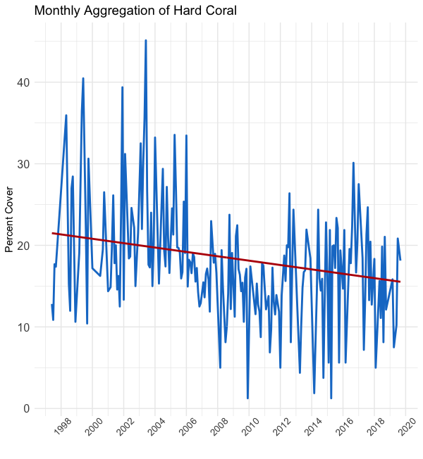
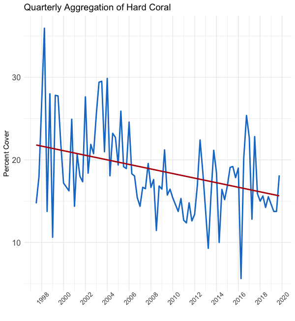
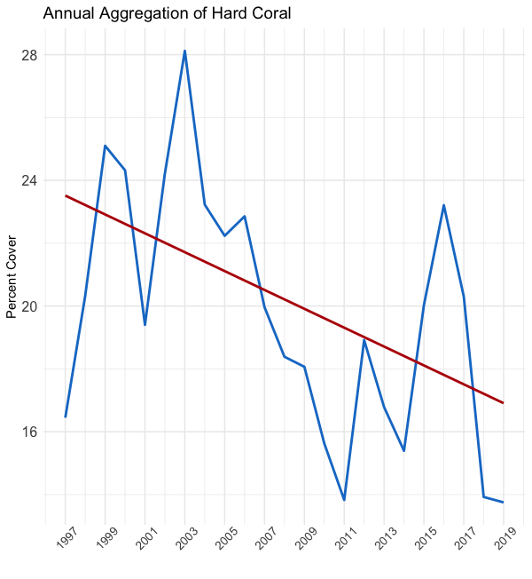
In the above figures, you can see the effect of averaging the data by monthly, quarterly, and yearly timeframes, respectively from left to right. As you “zoom out,” you reduce the variability in the data. Encompassed in this variability is both signal (good) and noise (bad). So, while the figure on the right shows the clearest trend, we’ve probably thrown out a lot of useful data.

在上圖中，您可以看到分別按從左到右的每月，每季度和每年時間范圍對數據進行平均的效果。 當您“縮小”時，可以減少數據的可變性。 這種可變性包括信號(好)和噪聲(壞)。 因此，盡管右圖顯示了最明顯的趨勢，但我們可能已經拋棄了許多有用的數據。

To encompass the maximum and minimum amount of information, we will fit our models to both the monthly and annually aggregated data.

為了涵蓋最大和最小信息量，我們將使模型適合于每月和每年匯總的數據。

Great, aggregation is done. On to our next manipulation: differencing.

很好，聚合完成了。 接下來的操作：差異化。

為什么需要與眾不同？ (Why do you need to difference?)

As a practical matter, most time series models assume something called stationary. In short, strong stationary means that each data point is pulled from the same theoretical probability distribution. But, because we cannot know what this population distribution looks like, we assume weak stationarity and develop proxies for consistency in the data, namely a constant mean, variance, and covariance over time.

實際上，大多數時間序列模型都采用稱為平穩的模型。 簡而言之，強平穩意味著每個數據點都從相同的理論概率分布中提取。 但是，由于我們不知道總體分布是什么樣子，因此我們假設平穩性較弱，并開發了數據一致性的代理，即隨時間推移的均值，方差和協方差。

If you recall in the aggregation plots above, we saw a trend, indicating the mean is not constant over time. Furthermore, while the variance is harder to eyeball, there appears to be less spread in the data from 2006 to 2012. After performing a Dickey-Fuller unit root test, our observations proved correct; the monthly and annually aggregated datasets are not stationary.

如果您回想起上面的聚合圖，我們看到了一個趨勢，表明平均值在一段時間內不是恒定的。 此外，雖然方差更難引起注意，但2006年至2012年的數據散布似乎較少。在進行了Dickey-Fuller單位根檢驗后，我們的觀察證明是正確的。 每月和每年匯總的數據集不是固定的。

So, to make the data useable for the ARIMA model, we will perform differencing, which simply involves subtracting each value from its prior value.

因此，為了使數據可用于ARIMA模型，我們將執行差分，這僅涉及從其先前值中減去每個值。

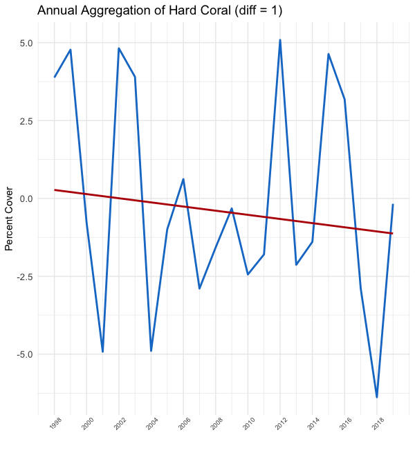
As you can see in the plots above, the y-axis values completely change from plot to plot. The leftmost plot, our un-differenced data, shows percent cover ranging from 12% to 28%. However, in the middle plot we are now working with the first difference, which shows the year over year change ranging from -6%-(+6%). The rightmost plot shows the second difference, or biannual change, with the y-axis range doubled as compared to our first-differenced plot.

如您在上面的圖中所看到的，y軸值在每個圖之間完全改變。 最左邊的圖(我們的未差異數據)顯示覆蓋率范圍從12％到28％。 但是，在中間圖中，我們正在處理第一個差異，該差異顯示逐年變化范圍為-6％-(+ 6％)。 最右邊的圖顯示了第二個差異，即半年變化，y軸范圍與我們的一階差異圖相比增加了一倍。

Not only does the y-axis change but the red trend line appears to flatten and the variance becomes more consistent over time. Lovely. This is what we wanted.

隨著時間的推移，不僅y軸發生變化，紅色趨勢線也趨于平坦，并且方差變得更加一致。 可愛。 這就是我們想要的。

To double check, we again use the unit root test and find that annual data with a difference of 2 passes the stationarity test.

為了再次檢查，我們再次使用單位根檢驗，發現相差2的年度數據通過了平穩性檢驗。

So, after performing similar steps for the monthly data, our datasets are now good to go. Ready to model?

因此，在對月度數據執行類似的步驟之后，現在可以使用我們的數據集了。 準備建模了嗎？

調整ARIMA模型 (Tuning the ARIMA Model)

ARIMA is three-part model that combines autoregressive (AR), integration (I), and moving average (MA) components. First, the AR component looks back at prior values in our data and uses them to fit the current value. Second, the I component simply means the data are differenced, the same concept we discussed above. And third, the MA component looks back a prior errors in our fit and uses them to predict the current value.

ARIMA是三部分模型，結合了自回歸(AR)，積分(I)和移動平均(MA)組件。 首先， AR組件回顧數據中的先前值，并使用它們來擬合當前值。 其次， I組件只是意味著數據有所不同，與我們上面討論的概念相同。 第三， MA組件會根據我們的擬合情況回顧先前的錯誤，并使用它們來預測當前值。

It’s not necessary to understand exactly how this works, but if you’re a knowledge loving person, this YouTube playlist does a great job of explaining ARIMA models (it’s also probably the best youtube tutorial I’ve ever seen).

不必確切了解其工作原理，但是如果您是一個知識淵博的人，那么此YouTube播放列表可以很好地解釋ARIMA模型(這也是我見過的最好的youtube教程)。

In its most basic form, ARIMA has three tuning parameters:

在最基本的形式中，ARIMA具有三個調整參數：

• p: how many prior values we use to fit the current value (i.e. for annual data, how many prior years of data should have an impact on the current year’s value).

  p ：我們使用多少個先前值來擬合當前值(即，對于年度數據，多少個先前年份的數據應該對當年的值產生影響)。

• d: how many times we difference.

  d ：我們相差多少次。

• q: how many prior errors we use to fit the current value.

  q ：我們使用多少個先前誤差來擬合當前值。

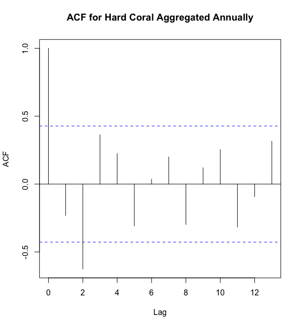
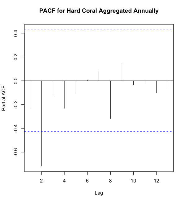
Note that we’ve already found d, so we just need to find p and q. To do this, we will use autocorrelation plots, which are shown below in Figures 8–9.

注意，我們已經找到了d ，所以我們只需要找到p和q即可。 為此，我們將使用自相關圖，如下圖8–9所示。

But why are there two plots? I thought there was only one variable: hard coral. That’s an outstanding point. If you’re a visual learner, check this out.

但是為什么會有兩個地塊？ 我以為只有一個變量：堅硬的珊瑚。 這是一個突出的觀點。 如果你是一個視覺學習者，檢查這出。

Either way, here’s a short explanation. The AutoCorrelation Function (ACF) plot on the left shows the correlation between hard coral now and hard coral at prior time periods, in this case years. The x-axis shows the number of years back we’re looking, and the y-axis shows the correlation between current hard coral and hard coral at the lagged time. The PartialAutoCorrelation Function (PACF) plot is very similar, however it also adjusts for the correlations of the values between the current time period and our lag by holding them constant. That’s why PACF is Partial; it doesn’t show all the correlations, whereas ACF does.

無論哪種方式，這里都有一個簡短的解釋。 左側的自相關函數(ACF)圖顯示了現在的硬珊瑚與以前時間段(在這種情況下為幾年)中的硬珊瑚之間的相關性。 x軸顯示了我們正在尋找的年份，y軸顯示了當前的硬珊瑚與滯后時間的硬珊瑚之間的相關性。 PartialAutoCorrelation Function(PACF)圖非常相似，但是它也通過將它們保持不變來調整當前時間段與我們的滯后值之間的相關性。 這就是為什么PACF是Partial； 它沒有顯示所有相關性，而ACF卻顯示了所有相關性。

In practice, we use the ACF plot to determine how many prior years are important for the AutoRegressive (AR) component. We then use the PACF to determine the Moving Average (MA) portion of the model. These values are called orders.

在實踐中，我們使用ACF圖來確定多少年對于自動回歸(AR)組件很重要。 然后，我們使用PACF來確定模型的移動平均(MA)部分。 這些值稱為訂單。

As you can see, the ACF plot has significant lags at 0 and 2, as indicated by a correlation greater than our significance threshold (blue dotted line). Note that a lag of 0 is simply the same time period, so a correlation of 1.0 makes sense. Applying the same process to the PACF plot, we can see a significant lag at 2. This leaves us with a p=2 and q=2. So, our annual ARIMA(p, d, q) would take the form ARIMA(2,2,2).

如您所見，ACF圖在0和2處有明顯的滯后，其相關性大于我們的顯著性閾值(藍色虛線)。 請注意，滯后0只是同一時間段，因此1.0的相關性是有意義的。 將相同的過程應用于PACF圖，我們可以看到在2處有明顯的滯后。這使我們剩下p = 2和q = 2 。 因此，我們的年度ARIMA( p ， d，q )將采用ARIMA(2,2,2)的形式。

Wow, that was a lot of setup, but now we’re well-equipped for fitting the data.

哇，這是很多設置，但是現在我們有足夠的設備來擬合數據。

培訓ARIMA (Training ARIMA)

Here we will be looking at 3 different models, namely:

在這里，我們將研究3種不同的模型，即：

1. ARIMA(2,2,2) with annual aggregation (developed above).
   具有年度匯總的ARIMA(2,2,2)(如上開發)。
2. ARMIA(3,1,1) with monthly aggregation.
   ARMIA(3,1,1)，每月匯總。
3. ARIMA(6,1,1) with monthly aggregation.
   每月匯總的ARIMA(6,1,1)。

To evaluate each models’ performance, we will use the squared correlation between the model’s fitted values and the true values; the r-squared closest to 1.0 is the winner.

為了評估每個模型的性能，我們將使用模型的擬合值和真實值之間的平方相關性。 最接近1.0的R平方是獲勝者。

每月匯總 (Monthly Aggregation)

Our ARIMA(3,1,1) model doesn’t perform great, exhibiting an r-squared valued of 0.156. We then run our ARIMA(6,1,1) model and get a very similar r-squared of 0.170. Unfortunately, it doesn’t look like we’re doing a great job of fitting.

我們的ARIMA(3,1,1)模型執行不佳，其r平方值為0.156。 然后，我們運行ARIMA(6,1,1)模型，得到非常相似的r平方0.170。 不幸的是，看起來我們并沒有做得很好。

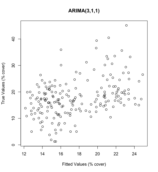
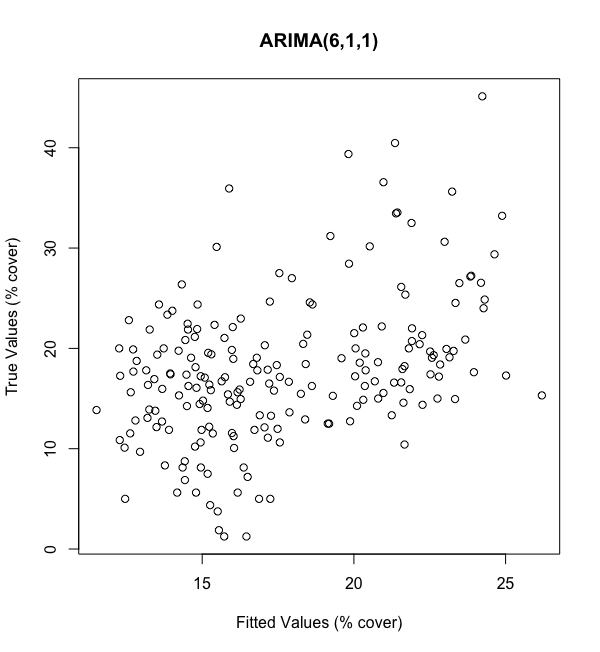
As show above in Figures 10–11, our poor fit is reflected by the lack of systematic trend between our fitted values (x-axis) and true values (y-axis). It also seems like our range of fitted values is far smaller than our true range; we’re off by about 15 percentage points in the high and low ends. So, not only is the fit bad, the scaling of the fit is bad as well.

如圖10-11所示，擬合值(x軸)和真實值(y軸)之間缺乏系統的趨勢反映了我們的擬合度較差。 看起來我們的擬合值范圍遠遠小于我們的真實范圍； 我們在高端和低端市場上下降了約15個百分點。 因此，不僅擬合度很差，而且擬合度也很差。

年度匯總 (Annual Aggregation)

Luckily, annual aggregation comes in to save the day with an r-squared of 0.689, indicating a very good fit (given the data).

幸運的是，年度匯總可以節省時間，且r平方為0.689，表明該數據非常合適(根據數據)。

As shown in the plot to the left, we have the true values in blue as compared to the fitted values in yellow. The fit looks pretty good, although it seems like the model is capturing the trend a little too late. Moreover, we don’t see the extreme scaling difference observed in the monthly models; instead, the fitted values are more extreme than the true data, as shown in 2003 and 2014. That being said, this appears to be a reasonable fit.

如左圖所示，藍色的真實值與黃色的擬合值相比。 擬合看起來不錯，盡管看起來該模型捕捉趨勢有點太晚了。 此外，我們沒有看到在每月模型中觀察到極端的比例差異； 相反，擬合值比真實數據更極端，如2003年和2014年所示。也就是說，這似乎是一個合理的擬合。

So, why did annual aggregation perform so much better? Well, it appears that our annual aggregation was able to smooth out the noise, allowing the model to accurately decipher trends. That being said, you can’t help but wonder what information was also thrown out by averaging.

那么，為什么年度匯總表現要好得多？ 好吧，看來我們的年度匯總能夠消除噪聲，從而使模型可以準確地解釋趨勢。 話雖這么說，您不禁要問平均也會拋出哪些信息。

In hopes of improving fits for both the monthly and annual models, the following variations were tested:

為了改善月度和年度模型的擬合度，對以下變化進行了測試：

• Adding a seasonal component with orders (3,0,1) and (6,0,1). Note this was only done for monthly data, but worsened the fit in both cases.
  添加訂單為(3,0,1)和(6,0,1)的季節性成分。 請注意，此操作僅針對月度數據進行，但兩種情況下的擬合均變差。

• Fitting with a predictor dummy variable: [1, 2, …, n-1, n]. This helped the fit significantly.

  擬合預測變量：[1,2，…， n-1 ， n ]。 這極大地幫助了擬合。

• Testing different p, d, q values (+/- 1), which worsened the fit.

  測試不同的p ， d ， q值(+/- 1)，這會使擬合度變差。

Ok, fairly confident we have maximized our training fit, let’s move on to forecasting.

好吧，非常有信心我們已經最大限度地提高了訓練水平，讓我們繼續進行預測。

ARIMA預測 (Forecasting With ARIMA)

Here we are going to predict the next 5 years of hard coral coverage using our annual ARIMA(2,2,2) model with the above dummy predictor.

在這里，我們將使用具有上述虛擬預測器的年度ARIMA(2,2,2)模型預測未來5年的硬珊瑚覆蓋率。

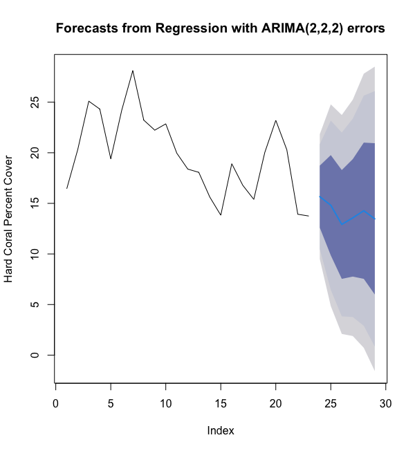
As indicated by the light blue trend line (in the dark shaded region), the forecasted percent cover is negative but not precipitous; the predicted value for 2025 is 13.46% cover. Moreover, the error bands are so large it’s impossible to make precise conclusions.

如淺藍色趨勢線所示(在深色陰影區域中)，預測的覆蓋率百分比為負，但并不險峻； 到2025年的預測價值是13.44％的覆蓋率。 而且，誤差帶太大，不可能得出準確的結論。

That being said, the error bands do provide interpretive power. The dark blue, dark grey, and light grey bands correspond to a 67%, 90%, and 95% confidence interval respectively. This means, for instance, that we are 67% confident that 5 years from now our percent cover will be between 5.99 and 20.95.

話雖如此，誤差帶確實提供了解釋力。 深藍色，深灰色和淺灰色帶分別對應67％，90％和95％的置信區間。 例如，這意味著我們有67％的信心，從現在開始的5年后，我們的覆蓋率范圍將在5.99到20.95之間。

To further interpret these confidence intervals, according to our model’s 95% confidence interval, we are 97.5% certain that we will not lose all hard coral in the Caribbean over the next 4 years. However, note that on the 5th year, this statement does not hold. Now looking at the upper side of our 95% confidence interval, we are 97.5% certain that in the next 5 years we will not surpass 29% cover, roughly corresponding to our our 22-year high observed in 2003.

為了進一步解釋這些置信區間，根據我們模型的95％置信區間，我們有97.5％的把握將在未來4年內不會失去加勒比海所有堅硬的珊瑚。 但是，請注意，在第5年，此聲明不成立。 現在來看我們95％的置信區間的上限，我們97.5％的人相信在未來5年中，我們的覆蓋率將不會超過29％，大致相當于我們在2003年所創的22年高點。

Well that was interesting, but a bit underwhelming. To produce a more precise forecast, we’ll have to try other techniques (hint: there will be a part 2).

嗯，這很有趣，但是有點讓人印象深刻。 為了產生更精確的預測，我們將不得不嘗試其他技術(提示：第2部分)。

結論 (Conclusion)

Three major takeaways from today’s analysis:

當今分析的三個主要收獲：

1. The Reef Check measures of hard coral do not provide much autoregressive signal until they are aggregated annually. That being said, we are exploring other aggregation methods, for instance our prior post.

   硬珊瑚的“珊瑚礁檢查”措施在每年進行匯總之前不會提供很多自回歸信號。 話雖如此，我們正在探索其他匯總方法，例如我們先前的post 。

2. Using univariate ARIMA, we can get a training r-squared of around 0.7 which is pretty good for such noisy data — just think about all the factors that can impact hard coral.
   使用單變量ARIMA，我們可以獲得約0.7的訓練R平方，對于這樣的嘈雜數據來說，這是非常好的-只需考慮可能影響硬珊瑚的所有因素即可。
3. However, our forecasts have extremely wide prediction intervals, meaning there’s a lot of uncertainty.
   但是，我們的預測具有非常寬的預測間隔，這意味著存在很多不確定性。

In following posts, we will add predictor variables to our time series model. We will also try other models to see if they produce better results. If you have ideas on where to go, leave a comment or reach out here.

在接下來的文章中，我們將預測變量添加到時間序列模型中。 我們還將嘗試其他模型，看看它們是否產生更好的結果。 如果您有去哪里的想法，請在此處發表評論或聯系。

資料來源 (Sources)

• Cryer, J. D., & Chan, K. (2011). Time series analysis with applications in R. New York: Springer.

  Cryer，JD，＆Chan，K.(2011年)。 時間序列分析及其在R中的應用 。 紐約：施普林格。

• Hyndman, R. J., & Athanasopoulos, G. (2018). Forecasting: Principles and practice. Melbourne: OTexts.

  Hyndman，RJ和Athanasopoulos，G.(2018年)。 預測：原理和實踐 。 墨爾本：OTexts。

• Warming, acidic oceans may nearly eliminate coral reef habitats by 2100. (n.d.). Retrieved September 02, 2020, from https://news.agu.org/press-release/warming-acidic-oceans-may-nearly-eliminate-coral-reef-habitats-by-2100/

  到2100年，變暖的酸性海洋幾乎可以消除珊瑚礁的棲息地。 于2020年9月2日從https://news.agu.org/press-release/warming-acidic-oceans-may-nearly-eliminate-coral-reef-habitats-by-2100/中檢索

The data were collected by Reef Check, a coral conservation non-profit that trains volunteer divers to collect marine data. With 1576 unique entries for the Caribbean ranging from 1997–05–24 to 2019–08–24, there were plenty of data points to conduct a TS analysis. However, the sampling variation differs greatly across location and time period. To combat this, we performed aggregation over time, however the difference in location still posed analysis problems. We largely ignored these, but analysis determining whether sampling location has a significant impact is required to derive conclusions.

數據是由珊瑚礁非營利組織Reef Check收集的，該組織培訓志愿潛水員收集海洋數據。 從1997–05–24到2019–08–24，在加勒比地區共有1576個唯一條目，其中有大量數據點可以進行TS分析。 但是，采樣變化在位置和時間段之間差異很大。 為了解決這個問題，我們隨時間進行了匯總，但是位置的差異仍然帶來了分析問題。 我們在很大程度上忽略了這些，但是需要分析確定采樣位置是否具有重大影響才能得出結論。

Here is the code.

這是代碼 。

Note: these are my findings. If you would like to contact me, leave a message here. All criticisms are welcome.

注意：這些是我的發現。 如果您想與我聯系，請在此處留言。 歡迎所有批評。